PostgreSQL Time Series Data Case: Automatic Compression of Time Series Data
This blog is a translation from the English version. You can check the original from here. We use some machine translation. We would appreciate it if you could point out any translation errors.
background
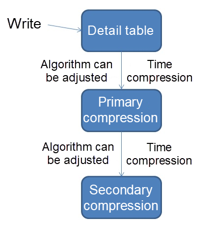
One of the most important features of time series databases is compression over time. For example, the data on the last day is compressed to points of about 5 minutes, and the data of the last week is compressed to points of about 30 minutes.
PostgreSQL's compression algorithm is customizable. For example, simple average compression, maximum compression, minimum compression, or compression based on revolving door compression algorithms.
[Implementation of rotating door data compression algorithm in PostgreSQL-Application of streaming compression in IoT, monitoring, and sensor scenarios](https://github.com/digoal/blog/blob/master/201608/20160813_01.md?spm=a2c65 .11461447.0.0.36311fe3ZBBoT1 & file = 20160813_01.md)
This article presents a simple compression scenario, such as compressing an RRD database into dimensions such as average, maximum, minimum, total, and number of records according to the time dimension.
It also introduces advanced SQL usage such as window queries, year-over-year comparisons, period comparison UDFs (including KNN calculations), and hourly uniform writes.
design
Detail table
create table tbl (
  id serial8 primary key,  -- primary key
  sid int,                 -- sensor ID
  hid int,                 -- indicator D
  val float8,              -- collected value
  ts timestamp             -- acquisition time
);

create index idx_tbl on tbl(ts);
Compressed table
1, 5 minute compression table
create table tbl_5min (
  id serial8 primary key,  -- primary key
  sid int,                 -- sensor ID
  hid int,                 -- indicator ID
  val float8,              -- inheritance, average, easy to do ring analysis
  ts timestamp,            -- inheritance, start time, easy to do ring analysis
  val_min float8,              -- minimum
  val_max float8,              -- maximum
  val_sum float8,              -- and
  val_count float8,            -- number of acquisitions
  ts_start timestamp,      -- interval start time
  ts_end timestamp         -- interval end time
);

alter table tbl_5min inherit tbl;
2, 30 minutes compression table
create table tbl_30min (
  id serial8 primary key,  -- primary key
  sid int,                 -- sensor ID
  hid int,                 -- indicator ID
  val float8,              -- inheritance, average, easy to do ring analysis
  ts timestamp,            -- inheritance, start time, easy to do ring analysis
  val_min float8,              -- minimum
  val_max float8,              -- maximum
  val_sum float8,              -- and
  val_count float8,            -- number of acquisitions
  ts_start timestamp,      -- interval start time
  ts_end timestamp         -- interval end time

);

alter table tbl_30min inherit tbl;
Compressed text for 3 to 5 minutes
with tmp1 as (
  delete from only tbl where ts <= now()-interval '1 day' returning *
)
insert into tbl_5min
  (sid, hid, val, ts, val_min, val_max, val_sum, val_count, ts_start, ts_end)
select sid, hid, avg(val) as val, min(ts) as ts, min(val) as val_min, max(val) as val_max, sum(val) as val_sum, count(*) as val_count, min(ts) as ts_start, max(ts) as ts_end from
tmp1
group by sid, hid, substring(to_char(ts, 'yyyymmddhh24mi'), 1, 10) || lpad(((substring(to_char(ts, 'yyyymmddhh24mi'), 11, 2)::int / 5) * 5)::text, 2, '0');
4, 30 minutes compressed text
with tmp1 as (
  delete from only tbl_5min where ts_start <= now()-interval '1 day' returning *
)
insert into tbl_30min
  (sid, hid, val_min, val_max, val_sum, val_count, ts_start, ts_end)
select sid, hid, min(val_min) as val_min, max(val_max) as val_max, sum(val_sum) as val_sum, sum(val_count) as val_count, min(ts_start) as ts_start, max(ts_end) as ts_end from
tmp1
group by sid, hid, substring(to_char(ts_start, 'yyyymmddhh24mi'), 1, 10) || lpad(((substring(to_char(ts_start, 'yyyymmddhh24mi'), 11, 2)::int / 30) * 30)::text, 2, '0');
demo
Write and distribute 100 million detailed test data in 10 days.
insert into tbl (sid, hid, val, ts) select random()*1000, random()*5, random()*100,   – 1000 sensors and 5 indicators per sensor.
  now()-interval '10 day' + (id * ((10*24*60*60/100000000.0)||' sec')::interval)   – push back for 10 days as the starting point + (id * time taken for each record)
from generate_series(1,100000000) t(id);
Compression scheduling for 2 to 5 minutes. For the data on the last day, the following SQL is scheduled every hour.
with tmp1 as (
  delete from only tbl where ts <= now()-interval '1 day' returning *
)
insert into tbl_5min
  (sid, hid, val, ts, val_min, val_max, val_sum, val_count, ts_start, ts_end)
select sid, hid, avg(val) as val, min(ts) as ts, min(val) as val_min, max(val) as val_max, sum(val) as val_sum, count(*) as val_count, min(ts) as ts_start, max(ts) as ts_end from
tmp1
group by sid, hid, substring(to_char(ts, 'yyyymmddhh24mi'), 1, 10) || lpad(((substring(to_char(ts, 'yyyymmddhh24mi'), 11, 2)::int / 5) * 5)::text, 2, '0');
Compression scheduling for 3 or 30 minutes. For the data of the last week, the following SQL is scheduled every hour.
with tmp1 as (
  delete from only tbl_5min where ts_start <= now()-interval '1 day' returning *
)
insert into tbl_30min
  (sid, hid, val_min, val_max, val_sum, val_count, ts_start, ts_end)
select sid, hid, min(val_min) as val_min, max(val_max) as val_max, sum(val_sum) as val_sum, sum(val_count) as val_count, min(ts_start) as ts_start, max(ts_end) as ts_end from
tmp1
group by sid, hid, substring(to_char(ts_start, 'yyyymmddhh24mi'), 1, 10) || lpad(((substring(to_char(ts_start, 'yyyymmddhh24mi'), 11, 2)::int / 30) * 30)::text, 2, '0');
Overview
- Group the time by interval and use integer division + multiplication.
For example For 5 minutes:
substring(to_char(ts, 'yyyymmddhh24mi'), 1, 10) || lpad(((substring(to_char(ts, 'yyyymmddhh24mi'), 11, 2)::int / 5) * 5)::text, 2, '0');
For 30 minutes:
substring(to_char(ts_start, 'yyyymmddhh24mi'), 1, 10) || lpad(((substring(to_char(ts_start, 'yyyymmddhh24mi'), 11, 2)::int / 30) * 30)::text, 2, '0')
- Generate evenly distributed time series data. By using the PG interval and generate_series, the write time can be evenly distributed among the corresponding intervals.
insert into tbl (sid, hid, val, ts) select random()*1000, random()*5, random()*100,   – 1000 sensors and 5 indicators per sensor.
  now()-interval '10 day' + (id * ((10*24*60*60/100000000.0)||' sec')::interval)   – push back for 10 days as the starting point + (id * time taken for each record)
from generate_series(1,100000000) t(id);
- One of the most important features of time series databases is that they are compressed over time. For example, the data for the last day is compressed to 5 minutes and the data for the last week is compressed to 30 minutes.
PostgreSQL's compression algorithm is customizable. For example, simple average compression, maximum and minimum compression, or compression based on revolving door compression algorithms.
This article presents a simple compression scenario, such as compressing an RRD database into average, maximum, minimum, total, number of records, and other dimensions according to the time dimension.
Add scheduling.
PostgreSQL Scheduled Task Method 2
[PostgreSQL Oracle Compatibility-DBMS_JOBS-Daily Maintenance-Timing Tasks (pgagent)](https://github.com/digoal/blog/blob/master/201305/20130531_01.md?spm=a2c65.11461447.0.0.36311fe3ZBBoT1&file= 20130531_01.md)
4, After compression, the interval, maximum value, minimum value, mean value, point value are included. These values can be used to draw the graphics.
- By combining with the window function of PG, you can easily draw a year-on-year graph or a graph that exceeds the period. An example of SQL is as follows.
Index and acceleration
create index idx_tbl_2 on tbl using btree (sid, hid, ts);
create index idx_tbl_5min_2 on tbl_5min using btree (sid, hid, ts);
create index idx_tbl_30min_2 on tbl_30min using btree (sid, hid, ts);
It is a complex type and returns the value of period-to-period comparison.
create type tp as (id int8, sid int, hid int, val float8, ts timestamp);
Gets a per-period value function that returns records for the specified SID and HID near a particular point in time, including the KNN algorithm.
create or replace function get_val(v_sid int, v_hid int, v_ts timestamp) returns tp as
$$

select t.tp from
(
select
(select (id, sid, hid, val, ts)::tp tp from only tbl where sid=1 and hid=1 and ts>= now() limit 1)
union all
select
(select (id, sid, hid, val, ts)::tp tp from only tbl where sid=1 and hid=1 and ts< now() limit 1)
) t
order by (t.tp).ts limit 1;

$$
 language sql strict;
Year-to-year, weekly, and monthly (these values can also be generated automatically to avoid calculations in each query).
select
sid,
hid,
val,
lag(val) over w1,                           --Same ratio
get_val(sid, hid, ts-interval '1 week'),    --Circumferential ratio
get_val(sid, hid, ts-interval '1 month')    --Lunar ratio
  from tbl         -- where ..., Time zone RBI.
window w1 as (partition by sid, hid order by ts)
- By combining with PG linear regression, you can draw a prediction index. The following example details this.
PostgreSQL Multiple Linear Regression-Stock Price Forecast 2
[Forecast using PostgreSQL linear regression analysis-Example 2 predicts closing stock price for the next few days](https://github.com/digoal/blog/blob/master/201503/20150305_01.md? spm = a2c65.11461447.0.0.36311fe3ZBBoT1 & file = 20150305_01.md)
PostgreSQL Linear Regression-Stock Price Forecast 1
Using Linear Regression Analysis in PostgreSQL-Implementing Data Prediction
- To facilitate development, the compression table is inherited by the detail table. This eliminates the need to write UNION SQL and allows you to get all the data (including compressed data) just by looking at the DETAIL table.
Related cases
Time-out streaming-Do not monitor data exceptions for incoming messages
PostgreSQL Streaming Statistics-"insert on conflict" Implementation Streaming Unique Visitor (Individual), Minimum, Maximum, Mean, Total, Count /20171123_02.md?spm=a2c65.11461447.0.0.36311fe3ZBBoT1&file=20171123_02.md)
HTAP Database PostgreSQL Scenarios and Performance Tests-32nd (OLTP) High-throughput Data I / O (Storage, Row Scan, No Index)-Atomic Asynchronous Batch Consumption (JSON + Functional Stream Computing)](https) //github.com/digoal/blog/blob/master/201711/20171107_33.md? spm = a2c65.11461447.0.0.36311fe3ZBBoT1 & file = 20171107_33.md)
HTAP Database PostgreSQL Scenarios and Performance Tests-27th (OLTP) IoT-FEED Logs, Stream Computing, Atomic Atomic Batch Consumption (CTE) /master/201711/20171107_28.md?spm=a2c65.11461447.0.0.36311fe3ZBBoT1&file=20171107_28.md)
[Real-time statistics of 10 million / s with PostgreSQL-based streaming pipeline DB](https://github.com/digoal/blog/blob/master/201510/20151015_01.md?spm=a2c65.11461447.0.0.36311fe3ZBBoT1&file = 20151015_01.md)