Tensorflow, it seems that even the eigenvalues of the matrix can be automatically differentiated

Synopsis

In Tensorflow, even if there is a place to find the diagonalization (eigenvalue) of the matrix in the middle when performing automatic differentiation by the gradient method, it seems that it can be minimized by the automatic differentiation and the gradient method without any problem.

I also added a method to manually ʻapply_gradientusingGradientTape and a method to minimize` the loss function by automatically differentiating it.

Version

• Tensorflow 2.1.0
• Python 3.7.3 (Anaconda)
• Windows 10

The point

When you prepare an appropriate 3-by-3 matrix $ A $ and calculate its eigenvalue $ \ lambda $, the derivative $ d \ lambda_0 / of each component of the matrix $ A $ with respect to the smallest eigenvalue $ \ lambda_0 $ When you want to calculate dA $ (it is a 3-by-3 matrix because it is for each component).

You can calculate $ d \ lambda_0 / dA $ with the following code. Since it is in Eager mode, use GradientTape () to grasp the calculation graph for differential calculation.

import tensorflow as tf

A = tf.random.uniform(shape=(3, 3))

with tf.GradientTape() as g:
    g.watch(A)
    val, vec = tf.linalg.eigh(A)
    val0 = val[0]
grad0 = g.gradient(val0, A)

print(A)
print(val)
print(grad0)

A

tf.Tensor(
[[0.6102723  0.17637432 0.38962376]
 [0.3735156  0.6306771  0.19141042]
 [0.34370267 0.7677151  0.4024818 ]], shape=(3, 3), dtype=float32)

val

tf.Tensor([-0.25994763  0.34044334  1.5629349 ], shape=(3,), dtype=float32)

grad0

tf.Tensor(
[[ 5.3867564e-04  0.0000000e+00  0.0000000e+00]
 [ 3.0038984e-02  4.1877732e-01  0.0000000e+00]
 [-3.5372321e-02 -9.8626012e-01  5.8068389e-01]], shape=(3, 3), dtype=float32)

Finally, since only the lower half is non-zero, it is speculated that ʻeigh` is using only the lower half.

Actually, the slice operation is performed as val0 = val [0], which is the main point. In other words, it does more than just calculate the eigenvalues. G.gradient (val, A) without cutting out one eigenvalue works fine, but ... I gave priority to the ease of explanation in mathematical formulas.

Also, val0 = val [0], but it is done in the GradientTape () environment. If all the operations that you want to connect the derivatives in this way are not done in this environment, g.gradient () will return None.

application

Since it is an automatic differentiation, it is possible to insert operations before and after. I will try it from now on.

Status

Prepare six values, arrange them in a symmetric matrix, and calculate the eigenvalues. Either this is true for a certain condition, or the error is calculated to be an error function, which is differentiated.

• Calculation before eigenvalue: Matrix composition
• Calculation after eigenvalue: Sum of error between eigenvalue and target value

By the way, like a machine learning library called Tensorflow, I will update the original value by the gradient method.

$ r $ holds 6 components of the 3x3 symmetric matrix, and $ t = (t_0, t_1, t_2) $ are the desired eigenvalues.

r = \left(r_0, r_1, \cdots, r_5\right)

Sort this

A_h=\left(\begin{array}{ccc}
\frac{1}{2} r_0 & 0 & 0 \\
r_3 & \frac{1}{2} r_1 & 0 \\
r_5 & r_4 & \frac{1}{2} r_2
\end{array}
\right)

A = A_h + A_h^T

Construct the matrix $ A $ as, and find the eigenvalues of it. Assuming that $ \ lambda = (\ lambda_0, \ lambda_1, \ lambda_2) $ is an array of three unique values of $ A $,

L = \sum_{i=0}^2\left(t_i - \lambda_i\right)^2

Is the loss function. To learn $ r $

\frac{\partial L}{\partial r_n} = \sum_{i,j,k}\frac{\partial A_{ij}}{\partial r_n}\frac{\partial \lambda_k}{\partial A_{ij}}\frac{\partial L}{\partial \lambda_k}

Is a necessary calculation. $ \ Frac {\ partial \ lambda_k} {\ partial A_ {ij}} $ in the middle is the derivative of the eigenvalues by the components of the matrix.

Analytical, it can be calculated by finding the solution $ \ lambda $ of $ \ det (A-\ lambda I) = 0 $, but honestly, if it exceeds 3D, it will be unmanageable unless it is a very sparse matrix. .. So, I rely on tensorflow, which can perform numerical calculations.

Manual differential call

First of all, it's annoying, but how to follow the process.

Preparation

    r = tf.Variable(initial_value=tf.random.uniform(shape=[6]))
    t = tf.constant([1.0, 1.0, 1.0])

r holds 6 components of the 3x3 symmetric matrix, and t is the desired eigenvalues. Here, a uniform random number is given to r as the initial value. Also, t is all 1.

Calculation for automatic differentiation

    with tf.GradientTape() as g:
        g.watch(r)
        A = 0.5*tf.linalg.diag(r[0:3])
        A = A + tf.pad(tf.linalg.diag(r[3:5]), [[0, 1], [1, 0]], "CONSTANT")
        A = A + tf.sparse.to_dense(tf.sparse.SparseTensor(indices=[[0, 2]], values=[r[5]], dense_shape=(3, 3)))
        A = A + tf.transpose(A)
        eigval, eigvec = tf.linalg.eigh(A)
        d = tf.reduce_sum((eigval - t)**2)

Since the processing from here is the target of automatic differentiation, we will do it in GradientTape.

There are two ways to substitute a specific component of ʻA from r, one is to use diag for introduction and the other is to use SparseTensor`.

I used tf.linalg.diag as a function to arrange three diagonal components and two components next to them. However, pad is used to arrange it in one place from the diagonal component, but the document introduces the option to arrange it in a place that is k offset from the diagonal using the k option. And when you use it

   A = A + tf.linalg.diag(r[3:5], k=1)

I can write, but somehow the k option did not work. So I use pad on purpose.

Also, as a way to set only one of $ r_5 $ at the corner of the matrix, Tensor does not have an index specification assign like numpy, so it is troublesome, but it is set by adding via a sparse matrix. Did.

After constructing ʻA, it is normal to calculate diagonalization ʻeigh and loss function. Here, the loss function $ L $ is d. I'm sorry it's complicated.

Derivative calculation

    grad_dr = g.gradient(d, r)

Again, d is the loss function $ L $. A tensor of length 6 is assigned to grad_dr. This has achieved the purpose of this article.

Update value

Use a suitable optimizer.

    opt = tf.keras.optimizers.Adam()
    opt.apply_gradients([(grad_dr, r), ])

Because differentiation can be used here

    opt.minimize(d, var_list=[r])

Then

TypeError: 'tensorflow.python.framework.ops.EagerTensor' object is not callable

I get the error. This is because the first argument d is required to be a function with no arguments that returns a loss function, not Tensor. This method will be described later.

Output example

For example, the initial r

<tf.Variable 'Variable:0' shape=(6,) dtype=float32, numpy=
array([0.12108588, 0.8856114 , 0.00449729, 0.22199583, 0.8411281 ,
       0.54751956], dtype=float32)>

At that time, ʻA` is

tf.Tensor(
[[0.12108588 0.22199583 0.54751956]
 [0.22199583 0.8856114  0.8411281 ]
 [0.54751956 0.8411281  0.00449729]], shape=(3, 3), dtype=float32)

It will be. Then the derivative $ \ frac {dL} {dr} $ of the loss function is

tf.Tensor([-1.757829   -0.22877683 -1.991005    0.88798404  3.3645139   2.1900787 ], shape=(6,), dtype=float32)

Was calculated. If you apply this like ʻopt.apply_gradients ([(grad_dr, r),]) , the value of r` will be

<tf.Variable 'Variable:0' shape=(6,) dtype=float32, numpy=
array([0.12208588, 0.8866114 , 0.00549729, 0.22099583, 0.8401281 ,
       0.5465196 ], dtype=float32)>

You can see that it is slightly different from the first value [0.12108588, 0.8856114, 0.00449729, 0.22199583, 0.8411281, 0.54751956].

To convergence

Why do you want to repeat it? If the optimization is successful, you will get a symmetric matrix with all 1 eigenvalues as set by t.

    while d > 1e-8:
        with tf.GradientTape() as g:
            g.watch(r)
            A = 0.5*tf.linalg.diag(r[0:3])
            A = A + tf.pad(tf.linalg.diag(r[3:5]), [[0, 1], [1, 0]], "CONSTANT")
            A = A + tf.sparse.to_dense(tf.sparse.SparseTensor(indices=[[0, 2]], values=[r[5]], dense_shape=(3, 3)))
            A = A + tf.transpose(A)
            eigval, eigvec = tf.linalg.eigh(A)
            d = tf.reduce_sum((eigval - t)**2)
        grad_dr = g.gradient(d, r)
        opt.apply_gradients([(grad_dr, r), ])
        print("---------------")
        print(r)
        print(eigval)
        print(d)

The d is the square error, which is repeated in a while loop until it falls below a certain level. When you do this

---------------
<tf.Variable 'Variable:0' shape=(6,) dtype=float32, numpy=
array([0.10630785, 0.18287621, 0.14753745, 0.16277793, 0.7271476 ,
       0.08771187], dtype=float32)>
tf.Tensor([-0.56813365  0.07035071  0.9315046 ], shape=(3,), dtype=float32)
tf.Tensor(3.3279824, shape=(), dtype=float32)
---------------
<tf.Variable 'Variable:0' shape=(6,) dtype=float32, numpy=
array([0.10730778, 0.18387613, 0.14853737, 0.16177836, 0.72614765,
       0.0867127 ], dtype=float32)>
tf.Tensor([-0.5661403   0.07189684  0.9309651 ], shape=(3,), dtype=float32)
tf.Tensor(3.3189366, shape=(), dtype=float32)
---------------
<tf.Variable 'Variable:0' shape=(6,) dtype=float32, numpy=
array([0.10830763, 0.18487597, 0.1495372 , 0.1607792 , 0.72514784,
       0.08571426], dtype=float32)>
tf.Tensor([-0.564147    0.07343995  0.9304282 ], shape=(3,), dtype=float32)
tf.Tensor(3.3099096, shape=(), dtype=float32)

The following is omitted

You can see that r and ʻA` are changing little by little. When it converges,

<tf.Variable 'Variable:0' shape=(6,) dtype=float32, numpy=
array([ 9.9999946e-01,  9.9999988e-01,  9.9999732e-01,  6.9962436e-05,
        4.2644251e-07, -1.1688111e-14], dtype=float32)>
tf.Tensor([0.9999294 0.9999973 1.0000702], shape=(3,), dtype=float32)
tf.Tensor(9.917631e-09, shape=(), dtype=float32)

have become. ʻA` seems to be an identity matrix. It was the same after several attempts, so it seems that finding a matrix with only one eigenvalue this way leads to an identity matrix.

If you count the number of loops, it seems that it takes thousands of steps such as 3066, 2341, 3035.

How to get automatic differentiation and update processing

The point is to use minimize ().

For the construction of the symmetric matrix ʻA`, refer to the "Calculations for automatic differentiation" section above.

    r = tf.Variable(initial_value=tf.random.uniform(shape=[6]))
    t = tf.constant([1.0, 1.0, 1.0])

    def calc_eigval(r):
        A = 0.5*tf.linalg.diag(r[0:3])
        A = A + tf.pad(tf.linalg.diag(r[3:5]), [[0, 1], [1, 0]], "CONSTANT")
        A = A + tf.sparse.to_dense(tf.sparse.SparseTensor(indices=[[0, 2]], values=[r[5]], dense_shape=(3, 3)))
        A = A + tf.transpose(A)
        eigval, eigvec = tf.linalg.eigh(A)
        return eigval
    def calc_loss(r):
        eigval = calc_eigval(r)
        d = tf.reduce_sum((eigval - t)**2)
        return d

    opt = tf.keras.optimizers.Adam()

    loss = lambda: calc_loss(r)

    while d > 1e-8:
        opt.minimize(loss, var_list=[r])
        print("---------------")
        print(r)
        print(calc_eigval(r))
        print(calc_loss(r))

calc_eigval is a function that returns an eigenvalue, and calc_loss is a function that calculates a loss function.

loss is a function that calculates a loss function based on the value of r at this point and returns its Tensor, givenloss (). The first argument of minimize requires a function without such an argument. So I was getting an error when I passed the d calculated by gradientTape to the minimize.

You can write calc_eigval in calc_loss, but I wanted to see how the eigenvalues changed during the loop, so I prepared another function. def calc_loss (r) and loss = lambda: calc_loss (r) are the points for using minimize. If you define calc_loss from the beginning with no arguments, you can pass it to minimize as it is. Anyway, now I don't have to manage it myself.

If you execute the above code as it is with the main function, the state of convergence will be output.

Other

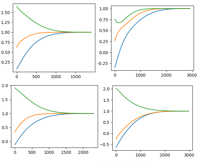
As a bonus, about 4 patterns that started the convergence of eigenvalues with random initial values. The lines are <font color = # 1f77b4> eigenvalue 1 </ font>, eigenvalue 2 </ font>, and <font color = # 2ca02c> eigenvalue 3 </ font>, respectively. The right end is 1, which is the goal of convergence, and you can see that it is working properly.