High-dimensional random number vector generation ~ Latin Hypercube Sampling / Latin hypercube sampling ~

Introduction

One of the problems in high-dimensional space is the spherical concentration phenomenon. The spherical concentration phenomenon is a phenomenon in which the density of points increases on the surface of a $ n $ hypercube in high-dimensional space. This phenomenon causes the problem that the number of samples near the center decreases when searching in high-dimensional space or using the Monte Carlo method. In this article, I would like to introduce Latin Hypercube Sampling, which is one of the sample methods to solve this problem. There is also a well-known sample method using the Sobol sequence.

Latin Hypercube Sampling Algorithm

When sampling $ M $ points in the $ n $ dimensional space, Latin Hypercube Sampling first divides each axis into $ M $ grids. In the figure below, an example is given when $ n = 2 $ and $ M = 5 $.

Then select cells one by one so that the rows do not cover each column.

Random numbers are generated in each selected cell and used as sample points.

This will prevent the selection of more than a few overlapping cells, so the average distance between a point and the closest point in space will probably be closer to the cell-to-cell centroid distance (actually different, but an image). In other words, the image is that it is easier to see the space more uniformly with fewer samples. For example, in the above two-dimensional example, the total number of squares at the edges (columns A, E, 1 row, 5 rows) is 16, and the number of internal squares is 9. Considering a simple probability, the probability that all samples will freeze on the outside is

\frac{{}_{16} C _{5}}{{}_{25} C _{5}} = \frac{16 \times 15 \times 14 \times 13 \times 12}{25 \times 24 \times 23 \times 22 \times 21}=\frac{8 \times 13}{5 \times 23 \times 11} \simeq 8.2 \%

It becomes. On the other hand, Latin Hypercube Sampling always samples from each column and does not allow duplicate rows, so the probability that all samples will freeze outside is $ 0 % $.

By the way, according to the manual calculation at hand, when $ n = 3, M = 5 $, it seems that everything is solidified outside with a probability of $ 29 % $ for uniform random numbers and $ 25.9 % $ for Latin Hypercube Sampling. It seems that there is not much difference if the number of divisions is small. (I will do a numerical experiment later.)

Latin Hypercube Sampling Code

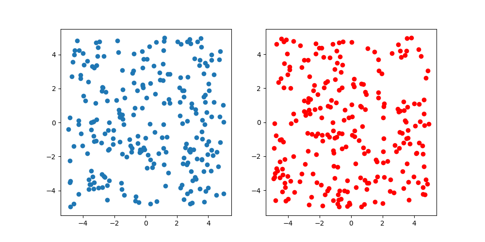
Just in case, compare with uniform random numbers. The number of samples is 250, blue is a uniform random number, and red is Latin Hypercube Sampling. Looking at the figure, it doesn't look like there is a difference, but it's two-dimensional, so it can't be helped. Since high-dimensional visualization is difficult, this is the end of this verification.

import numpy as np
import matplotlib.pyplot as plt 


n = 2
M = 250

lb, ub = -5., 5.

f = lambda x: (ub - lb) * x + lb
g = lambda x: (x - rng.uniform()) / M
rng = np.random.RandomState()
rs = f(rng.rand(M, n))

rnd_grid = np.array([rng.permutation(list(range(1, M + 1))) for _ in range(n)])
lhs = np.array([[f(g(rnd_grid[d][m])) for d in range(n)] for m in range(M)])


fig, ax = plt.subplots(1, 2, figsize=(10, 5)) 
ax[0].scatter(rs[:, 0], rs[:, 1]) 
ax[1].scatter(lhs[:, 0], lhs[:, 1], color="red")

plt.show()