Gradient method implementation 1

Introduction

It's been about a month since I booked this day on the Advent calendar, and it's almost Christmas. Somehow, I feel that this year has passed more quickly than usual. This time, I can write Python to some extent, but for those who do not know what kind of implementation will be concretely done by machine learning, I will send this as a Christmas gift from me in an easy-to-understand manner. Since the theoretical part and the practical part are mixed, please pick up and eat only the part that you can understand. Maybe you can still get a feel for it. Please also refer to here for an intuitive picture of machine learning in the previous article.

What is the gradient method?

The gradient method is one of the methods used for optimization. This gradient method is often used to find the weight $ W $ that gives the best output.

Specifically, previous The squared sum error shown

One of the methods to minimize is the gradient method, which uses differentiation to find the minimum value.

Implementation of differentiation

Let's start by implementing a one-dimensional derivative. The differential $ f ^ {\ prime} (x) $ of the function $ f (x) $ of $ x $ $ f ^ {\ prime} (x) = \ lim_ {h → 0} \ frac {f (x + h) --f (x)} {h} \ tag {2} It is defined by $. Derivative means the slope of the function $ f (x) $ at the point $ x $. For example, when the function is $ f (x) = x ^ 2 $ $ f ^ {\ prime} (x) = \ lim_ {h → 0} \ frac {(x + h) ^ 2- x ^ 2} {h} = 2x \ tag {3} $. The implementation is, for example: (Since only the code below is written for the main import destination, basically do not forget it after that.)

numerical_differentiation.py

import numpy as np
import matplotlib.pylab as plt

def nu_dif(f, x):
	h = 1e-4
	return (f(x + h) - f(x))/(h)

def f(x):
	return x ** 2
	
x = np.arange(0.0, 20.0, 0.1)
y = nu_dif(f, x)

plt.xlabel("x")
plt.ylabel("y")
plt.plot(x,y)
plt.show() 

This should plot the graph below $ y = f \ ^ {\ prime} (x) = 2x $. 

$ h $ is about $ 10 \ ^ {-4} $ to prevent rounding errors.

bonus

In the above numerical calculation, $$ f ^ {\ prime} (x) = \ lim_ {h → 0} \ frac {f (x + h) --f (x --h)} {2h} \ tag {4} $ Calculation like $ will improve the accuracy.

def nu_dif(f, x):
	h = 1e-4
	return (f(x + h) - f(x-h))/(2 * h)

Partial differential

Now that we have implemented the one-dimensional derivative, let's implement the multidimensional derivative. Here, for the sake of simplicity, we will differentiate in two dimensions. For a two-variable function $ f (x, y) $, the derivative of $ x, y $, that is, the partial derivative $ f_x, f_y 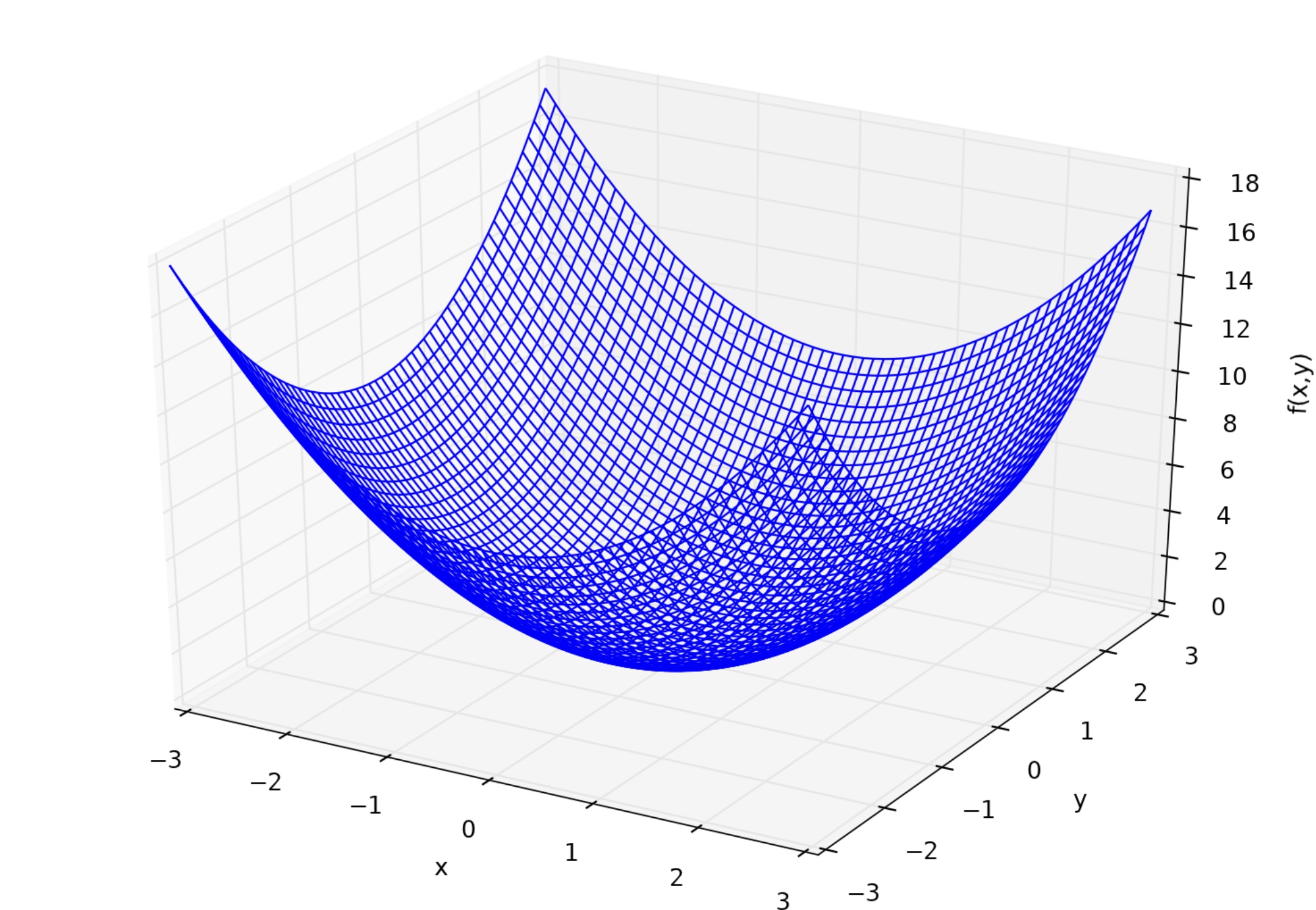, is defined as follows. $ f_x \ equiv \ frac {\ partial f} {\ partial x} = \ lim_ {h → 0} \ frac {f (x + h, y) --f (x, y)} {h} \ tag { 5} $ $ f_y \ equiv \ frac {\ partial f} {\ partial y} = \ lim_ {h → 0} \ frac {f (x, y + h) --f (x, y)} {h } \ tag {6} $$ Let's say that the function here is $ f (x, y) = x ^ 2 + y ^ 2 $.

Now let's implement partial differentiation as well. $ f_x = 2x, f_y = 2y $.

numerical_differentiation_2d.py

def f(x, y):
	return x ** 2 + y ** 2

def nu_dif_x(f, x, y):
	h = 1e-4
	return (f(x + h, y) - f(x - h, y))/(2 * h)
	
def nu_dif_y(f, x, y):
	h = 1e-4
	return (f(x, y + h) - f(x, y - h))/(2 * h)

Gradient

The gradient operator (nabla) for the three-variable function $ f (x, y, z) $ in 3D Cartesian coordinates is $ \ nabla f = \ bigg (\ frac {\ partial f} {\ partial x}, \ It is defined by frac {\ partial f} {\ partial y}, \ frac {\ partial f} {\ partial z} \ bigg) \ tag {7} $. Applying Nabla $ \ nabla $ to a scalar function gives a vector quantity. For example, when $ f (x, y, z) = x ^ 2 + y ^ 2 + z ^ 2 $, then $ \ nabla f = (2x, 2y, 2z) $. ** $-\ nabla f $ points to the minimum value of $ f $ (strictly the minimum value). ** Also, nablas can generally be extended to the $ n $ dimension. Illustrate $-\ nabla f = (-2x, -2y) $ for $ f (x, y) = x ^ 2 + y ^ 2 $ for intuitive understanding.  You can see that the $ xy $ planar vector $-\ nabla f $ points to the origin at every point. And the value at the origin is $ f (0,0) = 0 $, which is the minimum value of $ f $. The size of the arrow indicates the magnitude of the slope at that point.

Gradient method implementation

Thank you for your hard work. This completes all the math foundations needed to implement a simple gradient method. Now, let's implement a program that automatically finds the minimum value of the function. Arbitrary point Starting from $ \ boldsymbol {x} ^ {(0)} $ $$ \ boldsymbol {x} ^ {(k + 1)} = \ boldsymbol {x} ^ {(k)}-\ eta \ nabla It slides down to the point $ \ boldsymbol {x} ^ * $ which gives the minimum value according to f \ tag {8} $$. Here, $ \ eta $ is a hyperparameter that humans must specify in a quantity called the learning coefficient. $ \ eta $ must be adjusted appropriately so that it cannot be too large or too small. This time, the explanation about the learning coefficient is omitted.

Now, implement the gradient method and find the point $ \ boldsymbol {x} ^ * = (x ^ *, y ^ *) $ that gives the minimum value of $ f (x, y) = x ^ 2 + y ^ 2 $. Let's do it. As you already know, if you get $ \ boldsymbol {x} ^ * = (0,0) $, you are successful.

numerical_gradient.py

#Returns the gradient of f
def numerical_gradient(f, x):
	h = 1e-4
	grad = np.zeros_like(x)
	
	for i in range(x.size):
		tmp = x[i]
		x[i] = tmp + h
		f1 = f(x)
		x[i] = tmp - h
		f2 = f(x)
		grad[i] = (f1 - f2)/(2 * h)
		x[i] = tmp
		
	return grad	

#Gradient method
def gradient_descent(f, x, lr = 0.02, step_num = 200):
	for i in range(step_num):
		grad = numerical_gradient(f, x)
		x -= lr * grad
		
	return x
	
#define f
def f(x):
	return x[0] ** 2 + x[1] ** 2

#Output x
print(gradient_descent(f, np.array([10.0, 3.0])))

Result of $ \ boldsymbol {x} ^ {(0)} = (10,3), \ eta = 0.02, k = 0,1, \ ldots, 199 $ [ 0.00284608 0.00085382] Should be output. Since both $ x and y $ are about $ 10 ^ {-3} $, it can be said that they are almost $ 0 $.

Gradient method in machine learning

The outline and utility of the gradient method have been explained above. In machine learning, the key is how to find the optimal weight $ \ boldsymbol {W} $. The optimal weight is the loss function $ \ boldsymbol {W} $ that minimizes $ L $. The gradient method can be used as one of the methods to obtain this. The weight $ \ boldsymbol {W} $ is, for example, a $ 2 \ times2 $ matrix

\boldsymbol{W}=\left(\begin{array}{cc}
w_{11} & w_{12} \\
w_{21} & w_{22} 
\end{array}\right) \tag{9}

For the loss function $ L $ given in

\nabla L \equiv \frac{\partial L}{\partial \boldsymbol {W}}\equiv\left(\begin{array}{cc}
\frac{\partial L}{\partial w_{11}} & \frac{\partial L}{\partial w_{12}} \\
\frac{\partial L}{\partial w_{21}} & \frac{\partial L}{\partial w_{22}} 
\end{array}\right) \tag{10}

Calculate $ \ boldsymbol {W} ^ {(k + 1)} = \ boldsymbol {W} ^ {(k)}-\ eta \ nabla L \ tag {11} $ Applying the gradient method according to, we find $ \ boldsymbol {W} $, which gives the minimum value of $ L $. However, in most cases the obtained $ \ boldsymbol {W} $ does not give a minimum value of $ L $. It's like getting hooked on a pitfall before you get to your destination. The surface of $ L $ is often dented for various $ \ boldsymbol {W} $. To avoid this, there are some other ways that are a bit more complicated. I will write about this from the next time.

Summary

Thank you for reading this far. This time, I started by implementing a simple one-dimensional derivative using Python and extended it to multiple dimensions. Then, I introduced the gradient operator Nabla and learned the gradient method to find the minimum value of an arbitrary function using it. And finally, I told you that the gradient method can be used to reduce the loss function, which means that machine learning is more accurate. However, while the weights thus obtained are often extrema, we also find that the problem is that the loss function is not minimized, or optimized. From the next time onward, I will try to approach this problem in another way.

in conclusion

This time, I was blessed with the opportunity to be introduced by a friend and post to this Chiba University Advent Calendar 2019. It was a little difficult because I summarized it from a fairly rudimentary part, but I was able to write longer than usual and feel a sense of fatigue and accomplishment. In addition to my posts, various people are posting wonderful posts on various topics at various levels, so please take a look.