svm experiment 1

1. What kind of content

A set of 3 H x W pixel 1-channel images is given. Two sheets give a feature vector as a set, and one sheet is segmented and becomes an objective variable. The idea is to reproduce another segmented channel from two channels of data.

As a first idea, it would be nice if we could predict another channel from the pixel values of 2 channels in pixel units. Of course, the subject is to think about the convolution matrix and read up to a few pixel distances around it to make a prediction.

Further, the objective variable is classified according to whether the pixel value is equal to or more than the specified value, and it is expected that the pixel value is predicted by regression when the pixel value is less than the specified value.

For the time being, as a first attempt, I tried this classification.

The execution environment of python was separated using venv, and the necessary libraries were installed in it using pip.

python3 -m venv ./P
source P/bin/activate
pip install --upgrade pip
pip install --upgrade scikit-image

2. Data capture and confirmation

2.1 Reading / checking data

Two 1-channel images are read and stacked to form a 2-channel image. It should be one-dimensional and the class (0 or 1) should be compared with the pixel value [p1, p2].

I used scikit-image to read the image. Anything should have been fine this time. When you load the image, it becomes a H x W numpy array.

like this

>>> from skimage import io
>>> img = io.imread('train_images/train_hh_00.jpg')
>>> print(img.shape, img.dtype)
(8098, 11816) uint8
>>> print(img.max(), img.min(), img.mean(), img.std())
255 0 4.339263004581821 4.489037358487263
>>> print(img)
[[1 1 1 ... 6 7 5]
 [2 2 2 ... 6 8 8]
 [2 2 2 ... 7 8 9]
 ...
 [2 2 1 ... 6 7 8]
 [2 3 3 ... 8 9 8]
 [2 3 3 ... 8 9 8]]

After this

io.imshow(img)
io.show()

If you do, you can check it as an image

img *= 20

If you do something like that, you can expand the pixel value.

2.2 Confirmation of pixel value distribution of HH, HV images

I'm going to classify with this, so I'll visually check it properly.

Create an array of numpy arrays of the read HH, HV, annotation images and scatter plot them in 3D with matplotlib. When I try it, this is as slow as hell.

I can't plot everything very much, so I'll try to plot only a part by making it one-dimensional as follows.

import matplotlib.pyplot as plt

def reshape_them(img):
    rimg = list(map(lambda i: i.reshape([1, -1]), img))
    fig = plt.figure()
    ax = fig.add_subplot(111, projection='3d')
    ax.scatter(rimg[0][0][75500000:75510000], rimg[1][0][75500000:75510000], rimg[2][0][75500000:75510000], marker='o')
    ax.set_xlabel('X Label')
    ax.set_ylabel('Y Label')
    ax.set_zlabel('Z Label')
    plt.show()

The following results were obtained.

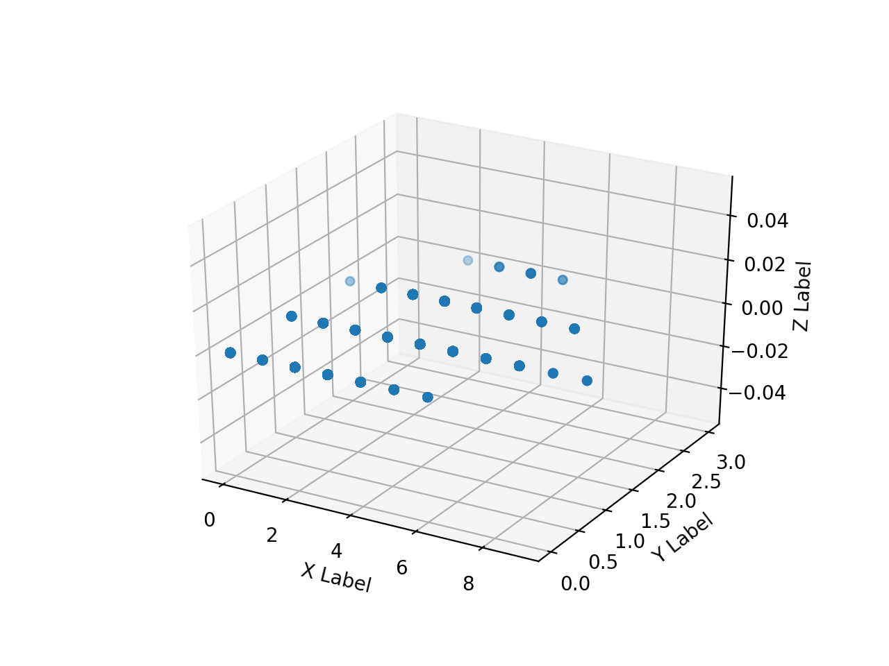
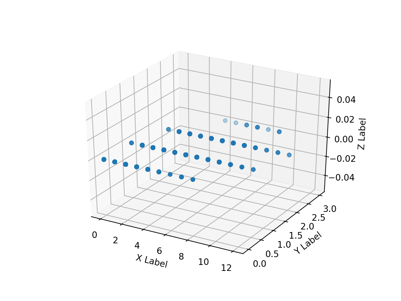
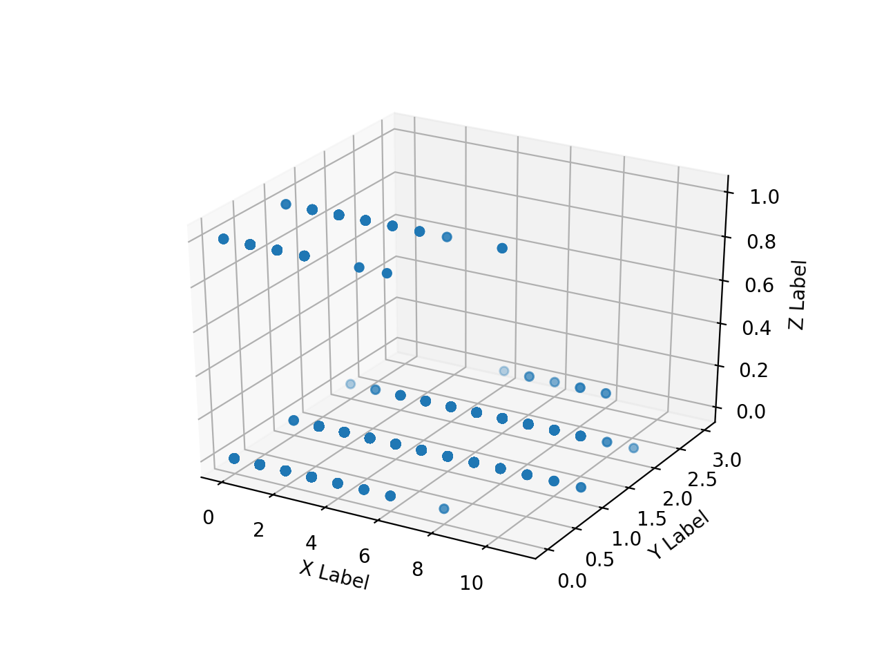
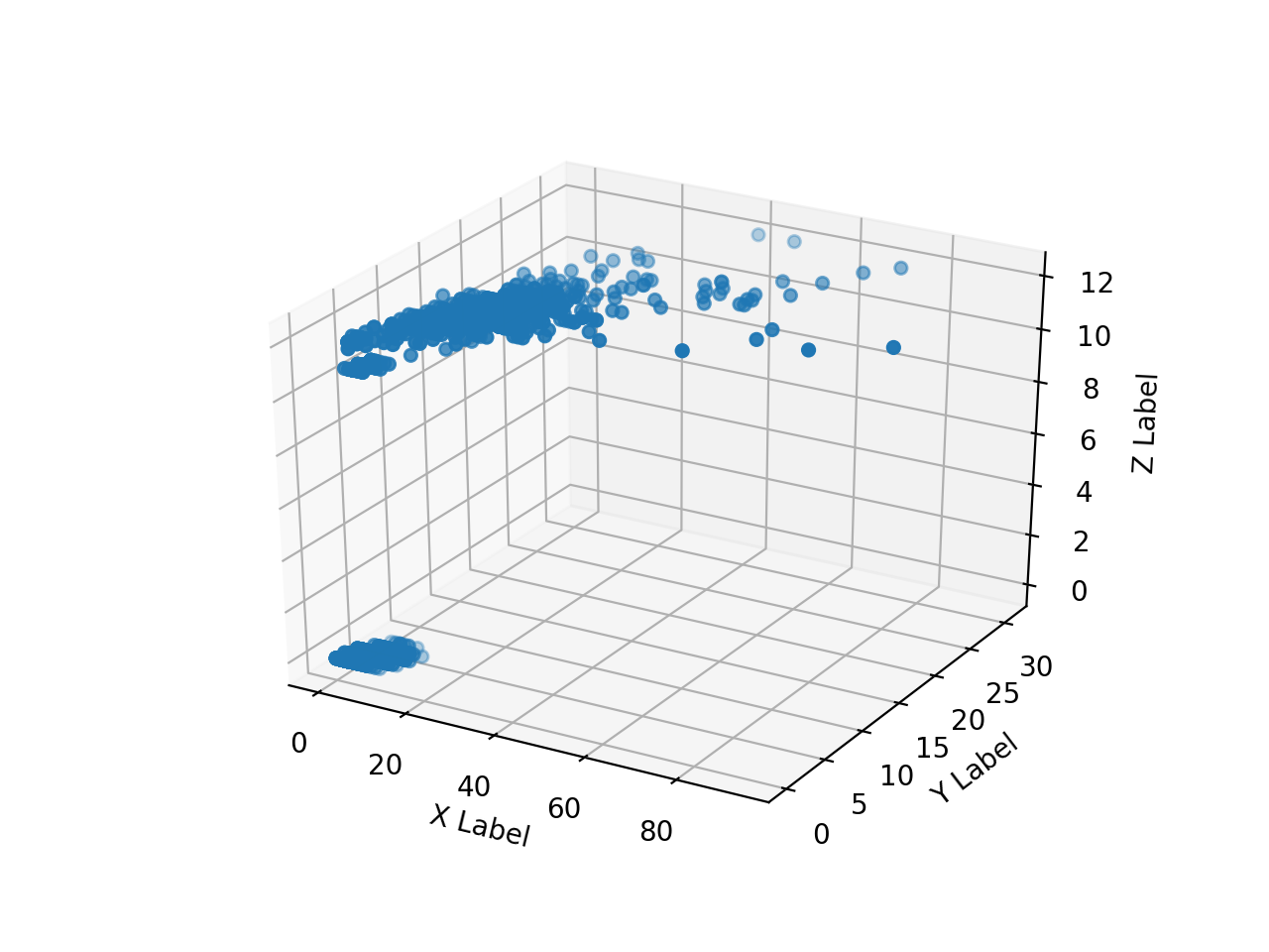
The array range of ʻax.scatter () is [0: 10000] , [500000: 510000] , [5500000: 5510000] , [755000000: 75510000] `, respectively.

Due to the convenience of the annotation image, the area where the pixel value (Z) of the teacher data takes some value is biased to the back. It can be seen that the same HH and HV values are divided into 2 classes. Therefore, it is reckless to classify only HH and HV into 2classes, but for the time being, let's see what can be obtained with this.

2.3 Create 3channel image

HH, HV Stack 1channel images to create 3channel images.

I thought it would be good to stack the numpy array mentioned above, but in the multi-channel image, the 2D array is not stacked for the number of channels, but A 1D array with the length of the number of channels was lined up in XY.

To make it, first make an array with 3 2D arrays arranged side by side (imgx), and then use transpose () to change the "axis" to make the channel direction the innermost (imgy).

    imgx = np.array([imgs[0], imgs[1], imgs[1]*0])
    imgy = imgx.transpose(1,2,0)
    imgz = imgy * 16
    io.imshow(imgz)
    io.show()

Since 3channel is required, \ * 0 is used to create and include all 0 planes. Also, since the pixel value is too small, it is corrected by \ * 16 so that it can be distinguished (imgz).

Since it's a big deal, I'll try to display it side by side with the original image.

    im21 = cv2.hconcat([gray2rgb(imgs[0]*16), gray2rgb(imgs[1]*16)])
    im22 = cv2.hconcat([gray2rgb(imgs[2]*16), imgz])

    im2 = cv2.vconcat([im21, im22])

    io.imshow(im2)
    io.show()

Gray2rgb () is used to match the number of channels when joining.

3. Classification --SVM

3.1 SVM

Let's get back to the story. After reading one H x W 1channel image, reshape it to 1 x H \ * W. If this is transposed by vstacking 2 images, the pixel values of 2 images are arranged for each pixel, and if it is also set with the annotation image reshaped to 1 x H \ * W, it seems that a classifier can be created with SVM.

import sklearn.svm
import joblib

from sklearn.model_selection import train_test_split
from sklearn.metrics import accuracy_score
import time

def reshape_and_calc(img):
    rimg = list(map(lambda i: i.reshape([1, -1]), img))
    print(rimg[0].shape, rimg[0].dtype, rimg[0].ndim)
    train = np.vstack((rimg[0], rimg[1])).transpose()
    label = rimg[2][0]
    print(train.shape, label.shape)
    train = train / 16.0 # [0..255]To[0..1)Equivalent to 16 times after
    label = np.where(label>10, 1, 0)
    print(train)
    print(label)

The scary thing is that the data eaten by training is an N x 2 matrix, but the label (objective variable) eaten by scikit-learn's svm is a 1 x N vector (so transpose () in the calculation of train". Is attached). Why is it different vertically and horizontally?

After this, feed the SVM classifier object entirely as shown below, and finally serialize itself with joblib.

    svm = sklearn.svm.SVC(kernel='rbf', random_state=0, gamma=0.10, C=10.0)
    svm.fit(train, label)
    joblib.dump(svm, 'svmmodel.sav')

However, this svm.fit () takes a lot of time and doesn't make any progress, so it gets stuck somewhere if it's really calculating. I can't tell if it's useless no matter how long I wait.

So, I'm wondering if it's okay to do it, but I'll try to cut out the data little by little and train it in sequence. The code below worked.

    train_X, test_X, train_y, test_y = train_test_split(train, label, train_size=0.8, random_state=1999)
    #print(train_X, test_X, train_y, test_y)
    print('data splitted', train_X.shape, test_X.shape, train_y.shape, test_y.shape)

    M = len(train_X)
    L=65536
    offset=0
    start_time = time.time()
    while offset < M:
        print('fitting', offset, '/', M, time.time() - start_time, "sec")
        L2 = min(offset+L, M)
        svm.fit(train_X[offset:L2], train_y[offset:L2])
        offset += L

    print('done')
    y_pred = svm.predict(test_X)
    print('Misclassified samples: %d' % (test_y != y_pred).sum())
    print('Accuracy: %.2f' % accuracy_score(test_y, y_pred))

Such a log remains.

fitting 76349440 / 76548774 706.0181198120117 sec
fitting 76414976 / 76548774 706.6317739486694 sec
fitting 76480512 / 76548774 707.2629809379578 sec
fitting 76546048 / 76548774 707.8376820087433 sec
done
Misclassified samples: 54996
Accuracy: 1.00

He handled 76,548,774 points in 707 seconds.

I suddenly became addicted to this when verification was done in a different file group in the first place, and I didn't want to train_test_split because I wanted to put all the data into learning.

3.2 SVM classification --Balance of positive and negative

train_test_split () cuts out a set for training and a set for verification for evaluation of learning results from one set of training data and labels. By the way, it seems that shuffle will be added at random. However, here, it is wasteful to turn a part for evaluation, and since evaluation is done in another file, suppose that you want to use the entire file for training data and do not use train_test_split ().

    train_X, test_X, train_y, test_y = train_test_split(train, label, train_size=0.8, random_state=1999)

If you simply insert the part of train, label into train_X, train_y, it will be rejected because the haste label data contains only correct examples.

ValueError: The number of classes has to be greater than one; got 1 class

Come to think of it, the source of this teacher data was a single image with pixel values, and the only different part of the class was the small area at the bottom of the image. If you pinch the pixel value from the top, only one class will be included if you do not advance considerably.

The improvement method is to extract the same number of pixels for both classes = 0 and = 1, combine them, randomly shuffle them just in case, and process them in order from the top, 65536 at a time. In order to extract the same number from both classes, the larger class needs random shuffle and is combined and shuffled again.

When I tried it, this was extremely slow. It's said that it's fast because it's numpy right away, but it's naturally slow if you do this.

In one file, the number of pixels was 95,685,968, of which 4,811,822 was a positive example, so 9,623,644 points were extracted by combining positive and negative. There are two values of HH and VV per point, and it will be a 64-bit floating point value when standardized with [0, 1), so 96M points x 2 x 8 bytes The input data was created by extracting 153.6M from 1.54G.

def reshape_them(imgs):
    rimg = list(map(lambda i: i.reshape([1, -1]), imgs))
    train = np.vstack((rimg[0], rimg[1])).transpose()
    teach = rimg[2][0]
    print(train.shape, teach.shape)
    train = train / 256.0
    teach = np.where(teach>10, 1, 0)

    return [train, teach]

def balance(data):
    train_x = data[0]
    train_y = data[1]
    mask = train_y == 1
    train_x_pos = train_x[mask]
    train_x_neg = train_x[np.logical_not(mask)]
    sample = min(len(train_x_pos), len(train_x_neg))
    train_y_balance = [1 for i in range(sample)] + [0 for i in range(sample)]
    print('shrink length to', len(train_y_balance))
    if len(train_x_pos) < len(train_x_neg):
        np.random.shuffle(train_x_neg)
    else:
        np.random.shuffle(train_x_pos)
    train_x_balance = np.concatenate([train_x_pos[:sample], train_x_neg[:sample]])
    print("shuffled and concatenated", train_x_balance.shape)

    Y = np.hstack([train_x_balance, np.array(train_y_balance).reshape([len(train_y_balance),1])])
    #print(Y.shape)
    np.random.shuffle(Y)
    print(Y[:,0:2], Y[:,2].transpose())

    return([Y[:,0:2], Y[:,2].transpose()])

def run(train_X, train_Y, model):
    print(train_X.shape, train_Y.shape)

    M = len(train_X)
    L=65536
    offset=0
    start_time = time.time()
    while offset < M:
        print('fitting', offset, '/', offset / M, time.time() - start_time, "sec")
        L2 = min(offset+L, M)
        #print(train_X[offset:L2], train_Y[offset:L2])
        model.fit(train_X[offset:L2], train_Y[offset:L2])
        offset += L

    print('done')

(X, Y) = reshape_them(imgs)
(X, Y) = balance([X, Y])

svm = sklearn.svm.SVC(kernel='rbf', random_state=0, gamma=0.10, C=10.0)
run(X, Y, svm)

3.3 SVM-After learning

The learning itself was done on AWS. When learning is finished

    joblib.dump(svm, modelfile)

The SVM object is serialized as Yasumura. Bring this to your local PC For the file at hand

    with open(modelfile, mode="rb") as f:
        svm = joblib.load(f)

        M = len(X)
        L=65536
        offset=0
        start_time = time.time()
        y_pred = []
        while offset < M:
            print('prediciting', offset, '/', offset / M, time.time() - start_time, "sec")
            L2 = min(offset+L, M)
            _Y = svm.predict(X[offset:L2])
            y_pred.append(_Y)
            #print('Misclassified samples: %d' % (Y[offset:L2] != _Y).sum())
            #print('Accuracy: %.2f' % accuracy_score(Y[offset:L2], _Y))
            offset += L

        predicted = np.concatenate(y_pred).reshape(imgs[2].shape)
        io.imshow(predicted)
        io.show()

        im2 = cv2.hconcat([predicted*10.0, imgs[2]*1.0])
        io.imshow(im2)
        io.show()

If you give the predicted value and combine it and return it to the image, it seems that you can judge how much it looks like as an image.

So, when I try it, the module name is slightly different between python on linux in the AWS environment and python on the local MacOS as shown below, and it cannot be read.

  File "/usr/local/Cellar/python/3.7.5/Frameworks/Python.framework/Versions/3.7/lib/python3.7/pickle.py", line 1426, in find_class
    __import__(module, level=0)
ModuleNotFoundError: No module named 'sklearn.svm._classes'

Certainly, if you look at the beginning of the serialization file, if you make it on AWS

00000000  80 03 63 73 6b 6c 65 61  72 6e 2e 73 76 6d 2e 5f  |..csklearn.svm._|
00000010  63 6c 61 73 73 65 73 0a  53 56 43 0a 71 00 29 81  |classes.SVC.q.).|
00000020  71 01 7d 71 02 28 58 17  00 00 00 64 65 63 69 73  |q.}q.(X....decis|
00000030  69 6f 6e 5f 66 75 6e 63  74 69 6f 6e 5f 73 68 61  |ion_function_sha|
00000040  70 65 71 03 58 03 00 00  00 6f 76 72 71 04 58 0a  |peq.X....ovrq.X.|

There is Ansco, but when I try to spit it on a mac

00000000  80 03 63 73 6b 6c 65 61  72 6e 2e 73 76 6d 2e 63  |..csklearn.svm.c|
00000010  6c 61 73 73 65 73 0a 53  56 43 0a 71 00 29 81 71  |lasses.SVC.q.).q|
00000020  01 7d 71 02 28 58 17 00  00 00 64 65 63 69 73 69  |.}q.(X....decisi|
00000030  6f 6e 5f 66 75 6e 63 74  69 6f 6e 5f 73 68 61 70  |on_function_shap|
00000040  65 71 03 58 03 00 00 00  6f 76 72 71 04 58 06 00  |eq.X....ovrq.X..|

There is no Ansco like. Well, there is a blur in such a place.

I couldn't help it, so I tried to predict it on AWS, but unlike learning, it's only one path calculation, but it's deadly slow. As mentioned above, there are many calculation points because there is no extraction to make the numbers positive and negative, but it is still slow.

ex73: prediciting 65929216 / 0.9993775530341474 9615.45419716835 sec
ex75: prediciting 70975488 / 0.9991167432331827 10432.654431581497 sec

It was a 2.8 hour course per file. Left predicted, right label