Translate Getting Started With TensorFlow

I decided to start TensorFlow. As a tutorial, MNIST etc. already has a Japanese translation of the predecessor, so I decided to translate Getting Started With TensorFlow (https://www.tensorflow.org/get_started/get_started) (as of March 11, 2017) that I could not find did.

Please point out any mistakes.

Getting Started With TensorFlow

With this guide you are ready to program in TensorFlow. Please Install TensorFlow before using this guide. To get the most out of this guide, you need to know the following:

--How to program in Python --What you know at least a little about arrays ――Ideally something about machine learning. If you don't know a little or at all, then this will be your first guide to read.

TensorFlow provides multiple APIs. The lowest level API (TensorFlow Core) gives you complete programming control. We recommend TensorFlow Core for machine learning researchers and others who need a finer level of control over their models. Higher level APIs are usually easier to learn and use than TensorFlow Core. In addition, these high-level APIs make repetitive tasks easier and more consistent across different users. High-level APIs like tf.contrib.learn help you manage datasets, estimates, and training and inference. Some of TensorFlow's high-level APIs (their method names include contrib) are under development. Some contrib methods may change or be deprecated in the next TensorFlow release.

This guide starts with TensorFlow Core. After that, I will explain how to implement the same model with tf.contrib.learn. Knowing the principles of TensorFlow Core provides a very good mental model of how things work internally when using a more compact high-level API.

Tensors The central unit of data in TensorFlow is a tensor. A tensor consists of a set of primitive values in the form of an array of arbitrary number of dimensions.

3 # Rank 0 tensor; This is a scalar with a shape of []. [1., 2., 3.] # Rank 1 tensor; This is a vector with shape [3]. [[1., 2., 3.], [4., 5., 6.]] # Rank 2 tensor; shape [2, 3] matrix. [[[1., 2., 3.]], [[7., 8., 9.]]] # shape [2, 1, 3], rank 3 tensor

TensorFlow Core tutorial Import TensorFlow

Below is a standard description of a TensorFlow import: import tensorflow as tf

This gives Python access to all TensorFlow classes, methods and symbols. Most of this document assumes that you have already done this.

Calculation graph

You might think that a TensorFlow Core program consists of two separate sections.

1. Build a computational graph
2. Run the calculation graph

** Computation Graph ** is a series of TensorFlow operations arranged on a multi-node graph. (A computational graph is a series of TensorFlow operations arranged into a graph of nodes.) Let's build a simple computational graph. Each node takes zero or more tensors as input and outputs one tensor. One type of node is a constant. All TensorFlow constants take no input and output the values stored inside them. You can create two floating point tensors node1 and node2 as follows:

node1 = tf.constant(3.0, tf.float32)

node2 = tf.constant (4.0) # Implicitly becomes tf.float32 print(node1, node2)

The result of the last print statement looks like this Tensor("Const:0", shape=(), dtype=float32) Tensor("Const_1:0", shape=(), dtype=float32)

Note that printing the node does not output the expected 3.0 or 4.0 values. Instead, they are nodes that output 3.0 and 4.0 respectively when evaluated. Computation graphs must be calculated within a ** session ** in order to properly evaluate the node. Sessions encapsulate control and state of the TensorFlow runtime.

The following code creates a Session object and then calls its run method to run the computational graph enough to evaluate node1 and node2. When I run the calculation graph in a session as below:

sess = tf.Session()
print(sess.run([node1, node2]))

You can see the expected 3.0 and 4.0 values:

[3.0, 4.0]

You can build more complex calculations by combining Tensor nodes with operations (operations are also nodes). For example, you can add two constant nodes to create a new graph as shown below:

node3 = tf.add(node1, node2)
print("node3: ", node3)
print("sess.run(node3): ",sess.run(node3))

The last two print statements print:

node3:  Tensor("Add_2:0", shape=(), dtype=float32)
sess.run(node3):  7.0

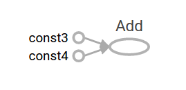
TensorFlow provides a utility called TensorBoard that can display images of computational graphs. Here is a screenshot showing how TensorBoard visualizes a graph:

At this rate, this graph is not particularly interesting because it always outputs the same result. Graphs can be parameterized to accept external input, known as ** placeholders **. ** Placeholders ** are prophecies to supply values later.

a = tf.placeholder(tf.float32)
b = tf.placeholder(tf.float32)
adder_node = a + b  # + provides a shortcut for tf.add(a, b)

The three lines above are like functions or lambdas. You define two input parameters (a and b) and then their operations. This graph can be evaluated with multiple inputs. By using the feed_dict parameter to identify the tensors that provide specific values for these placeholders.

print(sess.run(adder_node, {a: 3, b:4.5}))
print(sess.run(adder_node, {a: [1,3], b: [2, 4]}))

The output result is

7.5
[ 3.  7.]

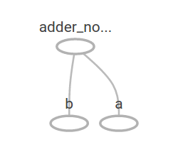
In TensorBoard, the graph looks like this:

You can create more complex computational graphs by adding other operations. For example

add_and_triple = adder_node * 3.
print(sess.run(add_and_triple, {a: 3, b:4.5}))

The output result is

22.5

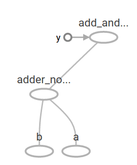
The above calculated graph looks like this on TensorBoard:

In machine learning, we usually want a model that can take ambiguous inputs like one of the above. To make the model trainable, we need to be able to modify the graph so that we can get new output for the same input. ** Variables ** allow you to add learnable parameters to your graph. They consist of type and initial value:

W = tf.Variable([.3], tf.float32)
b = tf.Variable([-.3], tf.float32)
x = tf.placeholder(tf.float32)
linear_model = W * x + b

The constant is initialized when you call tf.constant and its value does not change. In contrast, variables are not initialized when you call tf.Variable. In order for your TensorFlow program to initialize all variables, you must explicitly do something special:

init = tf.global_variables_initializer()
sess.run(init)

It is important to recognize that ʻinitis the handle of the TensorFlow sub-graph that initializes all global variables. Those variables are not initialized until you callsess.run`.

Since x is a placeholder, you can evaluate linear_model for several values x at the same time:

print(sess.run(linear_model, {x:[1,2,3,4]}))

The output is

[ 0. 0.30000001 0.60000002 0.90000004]

We created a model but don't know how good it is. In order to evaluate the model with training data, we need a y placeholder that provides the desired value and we need to write an error function.

The error function measures how far the current model is from the data provided. We will use the standard loss model for linear regression, which is the sum of the squares of the errors (deltas) between the current model and the data provided. linear_model-y creates a vector where each element corresponds to an example's error delta. Call tf.square to square those errors. Then use tf.reduce_sum to sum all the squared errors to make one scalar that extracts the errors of all the samples:

y = tf.placeholder(tf.float32)
squared_deltas = tf.square(linear_model - y)
loss = tf.reduce_sum(squared_deltas)
print(sess.run(loss, {x:[1,2,3,4], y:[0,-1,-2,-3]}))

The error value is

23.66

This can be remedied by manually reassigning the perfect values -1 and 1 for W and b. The variable is initialized to the value provided in tf.Variable, but can be changed by an operation like tf.assign. For example, W = -1 and b = 1 are the best parameters for our model. You can change W and b as follows:

fixW = tf.assign(W, [-1.])
fixb = tf.assign(b, [1.])
sess.run([fixW, fixb])
print(sess.run(loss, {x:[1,2,3,4], y:[0,-1,-2,-3]}))

The final print indicates that the error is zero.

0.0

I guessed the "perfect" values for W and b, but the whole point of machine learning is to automatically find the correct model parameters. We'll see how to achieve this in the next section.

tf.train API A complete discussion of machine learning is beyond the scope of this tutorial. However, TensorFlow provides ** optimizers ** that slowly change each variable to minimize the error function. The simplest optimizer is ** gradient descent **. It modifies each variable by the magnitude of the derivative for each variable in the error function. In general, manually calculating the symbolic derivative is tedious and error-prone. As a result, TensorFlow can calculate the derivative automatically by simply giving a description of the model using the tf.gradients function. Simply put, the optimizer usually does this for you. For example

optimizer = tf.train.GradientDescentOptimizer(0.01)
train = optimizer.minimize(loss)

sess.run(init) # reset values to incorrect defaults.
for i in range(1000):
  sess.run(train, {x:[1,2,3,4], y:[0,-1,-2,-3]})

print(sess.run([W, b]))

The last model parameter is: [array([-0.9999969], dtype=float32), array([ 0.99999082], dtype=float32)]

I was able to actually do machine learning! This simple linear regression doesn't require a lot of TensorFlow core code, but it does need more code to feed the model with more complex models and methods. Therefore, TensorFlow provides a higher level of abstraction for common patterns, structures, and features. You will learn how to use those abstractions in the next section.

Complete program

The full version of the trainable linear regression model is shown below:

import numpy as np
import tensorflow as tf

#Model parameters W = tf.Variable([.3], tf.float32) b = tf.Variable([-.3], tf.float32) #Model input and output x = tf.placeholder(tf.float32) linear_model = W * x + b y = tf.placeholder(tf.float32) #Error loss = tf.reduce_sum(tf.square(linear_model - y)) # sum of the squares #Optimizer optimizer = tf.train.GradientDescentOptimizer(0.01) train = optimizer.minimize(loss) #Training data x_train = [1,2,3,4] y_train = [0,-1,-2,-3] #Training loop init = tf.global_variables_initializer() sess = tf.Session() sess.run(init) # reset values to wrong for i in range(1000): sess.run(train, {x:x_train, y:y_train})

#Evaluate the accuracy of training curr_W, curr_b, curr_loss = sess.run([W, b, loss], {x:x_train, y:y_train}) print("W: %s b: %s loss: %s"%(curr_W, curr_b, curr_loss))

When run, it looks like this:

W: [-0.9999969] b: [ 0.99999082] loss: 5.69997e-11

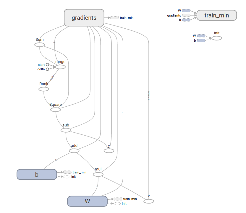
This more complex program can be visualized with TensorBoard

tf.contrib.learn

tf.contrib.learn is a high-level TensorFlow library that simplifies machine learning behavior. Includes:

--Run a training loop --Execute the evaluation loop --Manage datasets --Manage feeding

tf.contrib.learn defines many common models.

Basic usage

See how easy a simple linear regression program can be with tf.contrib.learn:

import tensorflow as tf

#NumPy is often used to read, manipulate, and preprocess data. import numpy as np

Declare a list of features. Right now I only use one real feature. More complicated and convenient

#There are many other types of columns features = [tf.contrib.layers.real_valued_column("x", dimension=1)]

#Estimator is a front end for training (fitting) and evaluation (estimation).

Linear regression, logistic regression, linear classification, logistic classification,

And like many neural network classifiers and regression

#There are many already defined types.

You can use a linear classification estimator with the following code.

estimator = tf.contrib.learn.LinearRegressor(feature_columns=features)

#TensorFlow contains many helper methods for loading and setting up datasets.

Here we use numpy_input_fn.

The number of batches (num_epochs) of required data and

Give the function how big each batch will be.

x = np.array([1., 2., 3., 4.])
y = np.array([0., -1., -2., -3.])
input_fn = tf.contrib.learn.io.numpy_input_fn({"x":x}, y, batch_size=4,
                                          num_epochs=1000)

By calling the # fit method and giving the training dataset

You can launch 1000 training steps.

estimator.fit(input_fn=input_fn, steps=1000)

Here, I will evaluate how good this model is. In a real example

I want to test a dataset using separate validation to prevent overfitting.

estimator.evaluate(input_fn=input_fn)

When run, the result looks like this

{'global_step': 1000, 'loss': 1.9650059e-11}

Custom model

tf.contrib.learn does not keep you in a predefined model. Let's say you want to create a custom model that isn't built into TensorFlow. You can keep the tf.contrib.learn dataset and high-level abstractions such as feeding and training. For illustration purposes, I'll show you how to create your own model equal to LinearRegressor using lower level knowledge of the TensorFlow API.

Use tf.contrib.learn.Estimator to define a custom model that works with tf.contrib.learn. In fact, tf.contrib.learn.LinearRegressor is a subclass of tf.contrib.learn.Estimator. Instead of subclassing ʻEstimator, we'll just provide ʻEstimator to the function model_fn, which tells tf.contrib.learn how it evaluates predictions, training numbers, and errors. .. The code looks like this:

import numpy as np
import tensorflow as tf

Declare a list of features. Right now I only use one real feature

def model(features, labels, mode):

Build a linear model to predict values

  W = tf.get_variable("W", [1], dtype=tf.float64)
  b = tf.get_variable("b", [1], dtype=tf.float64)
  y = W*features['x'] + b

#Error subgraph loss = tf.reduce_sum(tf.square(y - labels)) #Training subgraph global_step = tf.train.get_global_step() optimizer = tf.train.GradientDescentOptimizer(0.01) train = tf.group(optimizer.minimize(loss), tf.assign_add(global_step, 1)) #ModelFnOps for proper functionality (funcrionality)

Combine the subgraphs you have created so far

  return tf.contrib.learn.ModelFnOps(
  mode=mode, predictions=y,
  loss=loss,
  train_op=train)

estimator = tf.contrib.learn.Estimator(model_fn=model)

#Dataset definition x = np.array([1., 2., 3., 4.]) y = np.array([0., -1., -2., -3.]) input_fn = tf.contrib.learn.io.numpy_input_fn({"x": x}, y, 4, num_epochs=1000)

#Training estimator.fit(input_fn=input_fn, steps=1000) #Evaluate the model print(estimator.evaluate(input_fn=input_fn, steps=10))

The execution result will be as follows

{'loss': 5.9819476e-11, 'global_step': 1000}

Note that the content of the custom model () function is very similar to a loop that manually trains a model from a low-level API.

Next step

I have a useful basic knowledge of TensorFlow. We have prepared some tutorials to help you learn more. If you are a beginner in machine learning, MNIST for beginners, otherwise Deep MNIST for experts See (/ get_started / mnist / pros).

Unless otherwise noted, the content of this page is Creative Commons Attribution 3.0 License and the code is Apache 2.0 License. It is licensed under .apache.org/licenses/LICENSE-2.0). See Site Policies for more information. Java is a registered trademark of Oracle and its affiliates.

Last updated March 8, 2017