[Python, Julia] 3D display in Jupyter-Mayavi library
[Memo 2019/12/24. Thank you for "Like" and "Stock" this article even at the end of 2019. The basics are the same as the following, but since it is the era of Python 3.x and Julia 1.x, please keep track of the latest situation. ]
Jupyter Advent calendar 2016 This is the article on the 12th day. You can view 3D graphics in Jupyter. Use Python's Mayavi library. Mayavi is a 3D graphics display library for Python. The graphics engine is vtk, which was developed with visualization in the field of science and technology in mind. If you watch the demo, you can see what kind of picture you can draw. -> Demo, [MRI example](http://docs.enthought.com/mayavi/mayavi/auto/example_mri.html? highlight = mri)
set the table
In order for Jupyter to display the output of the Mayavi library, the following two conditions must be met.
--The Mayavi package is available in the Python kernel called by Jupyter. --The nbextension for Mayavi is installed on jupyter.
Actually, this setting is the most difficult. If you are interested in the display results, you can skip the rest of this section. Below, we will try to build an environment on Mac OSX using the conda environment.
(1) Install Python2 and Mayavi
Mayavi's anaconda package is only available in python 2, so install the latest version of Python 2.7 at the moment. An overview of Python environment construction is summarized in Python environment construction 2016 for those who aim to become data scientists. Be careful when dealing with multiple conda environments, but the first of 3 types of workarounds for activate collision problem when coexisting pyenv and anaconda In other words, I operate with the policy of "installing anaconda using pyenv and then not using pyenv". After installing pyenv and anaconda as described in the article, create a conda environment for Mayavi (hereinafter referred to as py27mayavi).
conda install -n py27mayavi numpy jupyter mayavi=4.4
source activate py27mayavi
Mayavi is sensitive to the version of the library you use. The latest version of Mayavi is 4.5, but I feel that the previous 4.4 is stable. After adding Mayavi, make sure that Mayavi works from Python. If you see a 3D picture, you are successful.
from mayavi import mlab
mlab.test_plot3d()
(2) Enable the conda environment with Jupyter.
Make it possible to call the conda environment py27mayavi created in (1) from Jupyter.
The setting method for switching between multiple kernels (conda environment) from the running Jupyter is described in the article How to easily switch the virtual environment created by Conda on Jupyter. It is introduced in yoppe / items / 38005f415a5b8b884c7d # comment-a914efbb53ef23992ba1). For example, as shown in the figure below, it is convenient because you can select the kernel to boot with New Notebook.

(3) Add nbextension to Jupyter
nbextensions is also installed using conda. Refer to here-> https://github.com/ipython-contrib/jupyter_contrib_nbextensions
conda install -n py27mayavi -c conda-forge jupyter_contrib_nbextensions
According to Using Mayavi in Jupyter notebooks, to install nbextensions for Mayavi,
jupyter nbextension install --py mayavi --user
It says to type in, but this didn't work. However, when I start mlab.init_notebook from within Jupyter (see below), nbextensions for Mayavi exist, so let's say the result is okay.
The simplest example Python
Start Jupyter from a shell (command line, terminal).
jupyter notebook
```
Use the conda environment where Mayavi is installed as the kernel and use New notebook. Let's call Mayavi.
Jupyter Notebook below: https://gist.github.com/anonymous/2c85c265cbee3c4485cfe39239593a11
````python
from mayavi import mlab
mlab.init_notebook()
s=mlab.test_plot3d()
s
```
To display objects in Mayavi, you typically use the `mayavi.mlab` module. `mlab.init_notebook ()` is a "magic" for outputting Mayavi images on Jupyter.
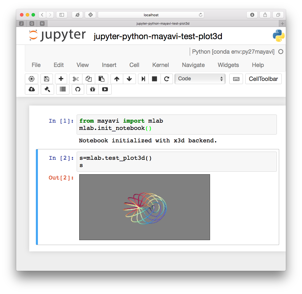
In the output cell ʻOut [*]`, a window for 3D display opened and the 3D object was displayed. You can rotate and scale the object by holding down the left button and moving the mouse, and you can move the object by holding down the Shift key and the left button.
# Display mechanism
I think that the mechanism of 3D display is as follows.
After `mlab.init_notebook ()`, the message` Notebook initialized with x3d backend` "notebook was set to handle 3D scenes in` x3d` format "was output, but` x3d` It is the successor to VRML (Virtual Reality Modeling Language), a format for describing 3D scenes. If Mayavi outputs a 3D scene in `x3d` format, Jupyter notebook will draw the 3D image in your web browser. HTML5-compliant modern browsers take advantage of WebGL, which has the ability to display a subset of the 3D graphics standard OpenGL.
# Ironclad: Output a Mayavi object
Next, let's write a simple program. The [test program](http://docs.enthought.com/mayavi/mayavi/auto/mlab_helper_functions.html#surf) of the surface drawing function `surf`.
Jupyter Notebook below: https://gist.github.com/anonymous/954fdf1bebc9802a3e035092c1ac50ff
```python
import numpy as np
def f(x, y):
return np.sin(x + y) + np.sin(2 * x - y) + np.cos(3 * x + 4 * y)
x, y = np.mgrid[-7.:7.05:0.1, -5.:5.05:0.05]
from mayavi import mlab
mlab.init_notebook()
s = mlab.surf(x, y, f)
s
```
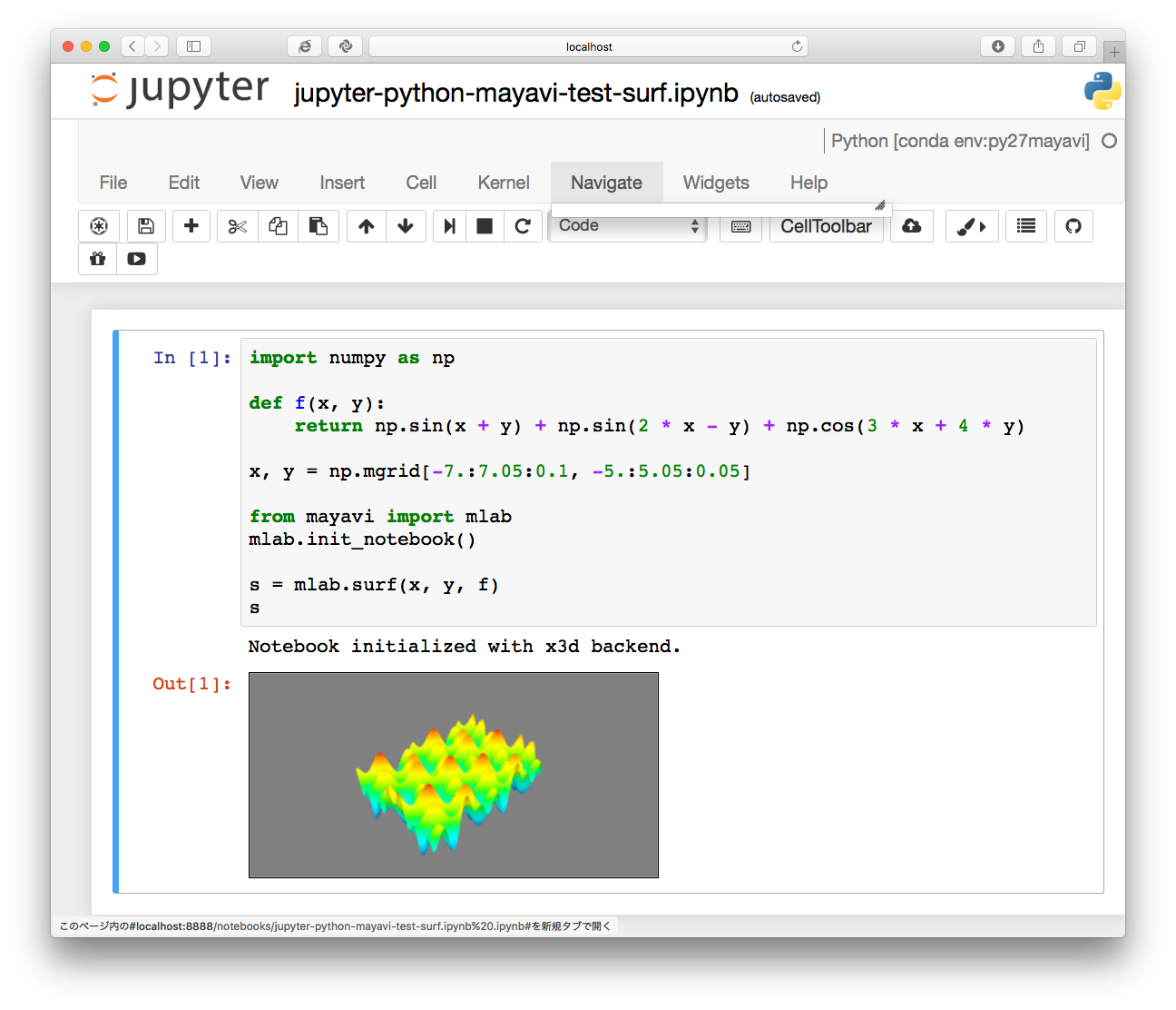
The state of the function `f` is drawn.
To get this drawing result, you need the `s` written on the last line. If you remove it, nothing will be drawn. In other words, when you output a Mayavi object to the Jupyter output cell, it seems to be drawn in 3D.
With that in mind, here's an example:
Jupyter Notebook below: https://gist.github.com/anonymous/f55d3291bf778bd5fef98e0741d82d65
```python
import numpy as np
np.random.seed(12345)
x = 4 * (np.random.random(500) - 0.5)
y = 4 * (np.random.random(500) - 0.5)
z = np.exp(-(x ** 2 + y ** 2))
from mayavi import mlab
mlab.init_notebook()
mlab.figure(1, fgcolor=(0, 0, 0), bgcolor=(1, 1, 1))
pts = mlab.points3d(x, y, z, z, scale_mode='none', scale_factor=0.2)
mesh = mlab.pipeline.delaunay2d(pts)
surf = mlab.pipeline.surface(mesh)
mlab.view(47, 57, 8.2, (0.1, 0.15, 0.14))
mlab.show()
mesh
surf
```
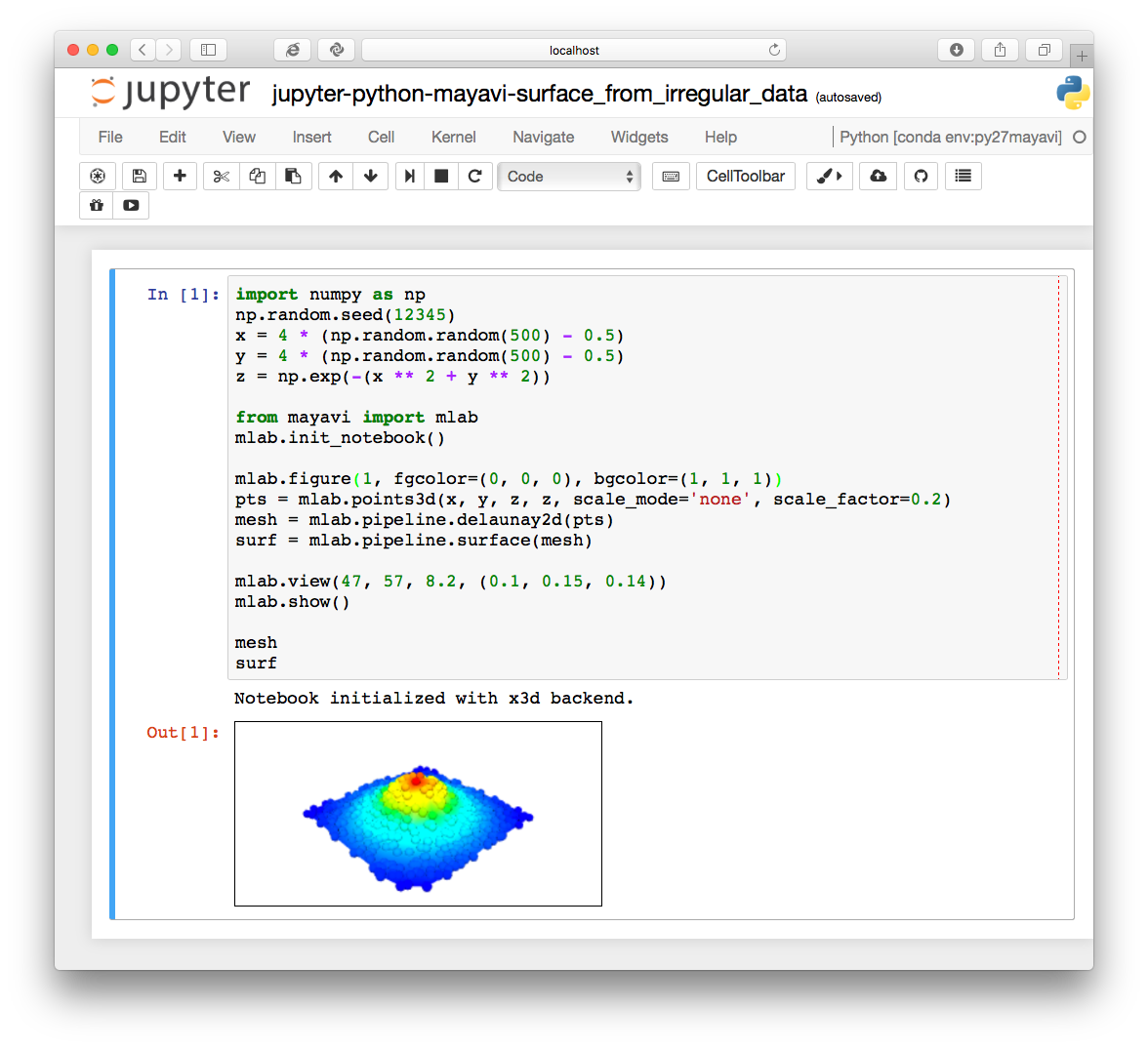
To get 3D drawing, we need the last two lines of the program, `mesh` and` surf`. If you output Mayavi objects at the end of the program, Jupyter will pick them up and draw them in 3D.
# Julia But Mayavi on Jupyter
[Julia](http://julialang.org) is a new programming language that can be executed interactively but still enjoys extremely high performance of numerical calculations.
In my article I wrote last week, I explained how to use Mayavi with Julia and how to operate the conda environment from Julia.
* [Use 3D plot library MayaVi from Julia](http://qiita.com/tenfu2tea/items/b38c3c36c4771c963cc6)
* [Add conda package from Julia](http://qiita.com/tenfu2tea/items/d2ac1427eaed7a548287)
## The simplest example Julia
Here's the simplest example of calling Mayavi inside Jupyter.
Jupyter Notebook below:
https://gist.github.com/anonymous/b991896af47ac1ef3fed630b0922bd7a
```julia
using PyCall
@pyimport mayavi.mlab as mlab
mlab.init_notebook()
mlab.test_points3d()
```
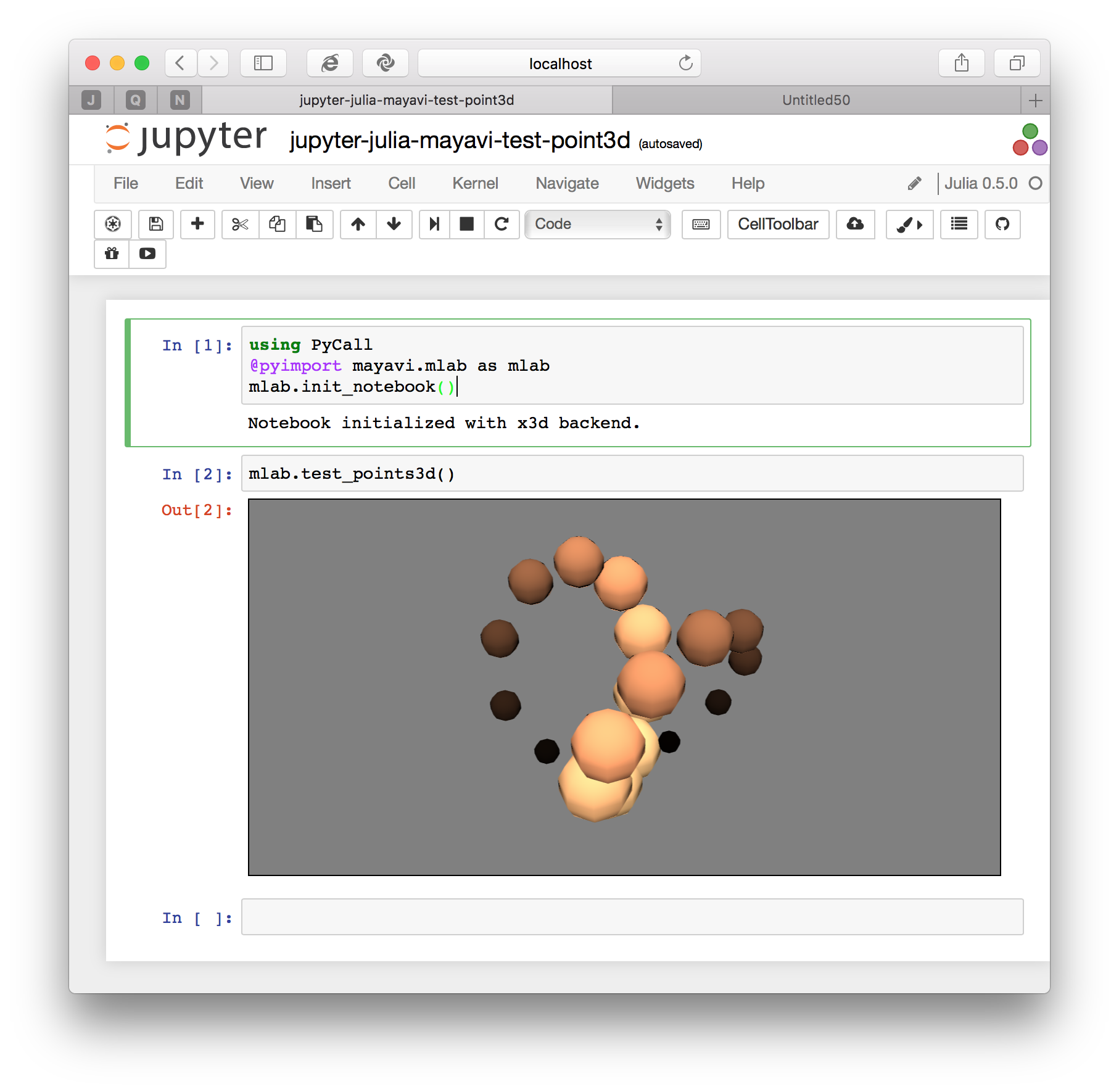
To use a Python module from Julia, do ʻusing PyCall` and then load the Python module you want to use with` @ pyimport`. The Python ʻimport` instruction is equivalent to Julia's `@ pyimport` instruction. Objects loaded with `@ pyimport` are of Julia type, so you can call them as they are from within Julia.
```python
import mayavi.mlab as mlab # Python
@pyimport mayavi.mlab as mlab # Julia
```
Spherical Harmonics
[Example](http://qiita.com/tenfu2tea/items/b38c3c36c4771c963cc6#spherical_harmonics) of Spherical Harmonics introduced in [My sentence](http://qiita.com/tenfu2tea/items/b38c3c36c4771c963cc6) , Try running it on Jupyter.
Jupyter Notebook below:
```julia
phi = [ u1 for u1 in linspace(0,pi,101), v1 in linspace(0,2*pi,101) ]
theta = [ v1 for u1 in linspace(0,pi,101), v1 in linspace(0,2*pi,101) ]
r = 0.3
x = r * sin(phi) .* cos(theta)
y = r * sin(phi) .* sin(theta)
z = r * cos(phi)
using PyCall
@pyimport scipy.special as spe
@pyimport mayavi.mlab as mlab
mlab.init_notebook("x3d")
mlab.figure(1, bgcolor=(1, 1, 1), fgcolor=(0,0,0), size=(400, 300))
mlab.clf()
mlab.view(90, 70, 6.2, (-1.3, -2.9, 0.25))
u=false
for n in 1:6-1, m in 0:n-1
s = real( spe.sph_harm(m, n, theta, phi) )
mlab.mesh(x - m, y - n, z, scalars=s, colormap="jet")
s[s .< 0] *= 0.97
s /= maximum(s)
u = mlab.mesh(s .* x - m, s .* y - n, s .* z + 1.3,
scalars=s, colormap="Spectral" )
u
end
u
```
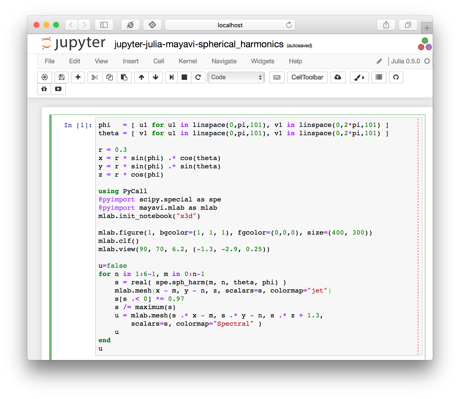
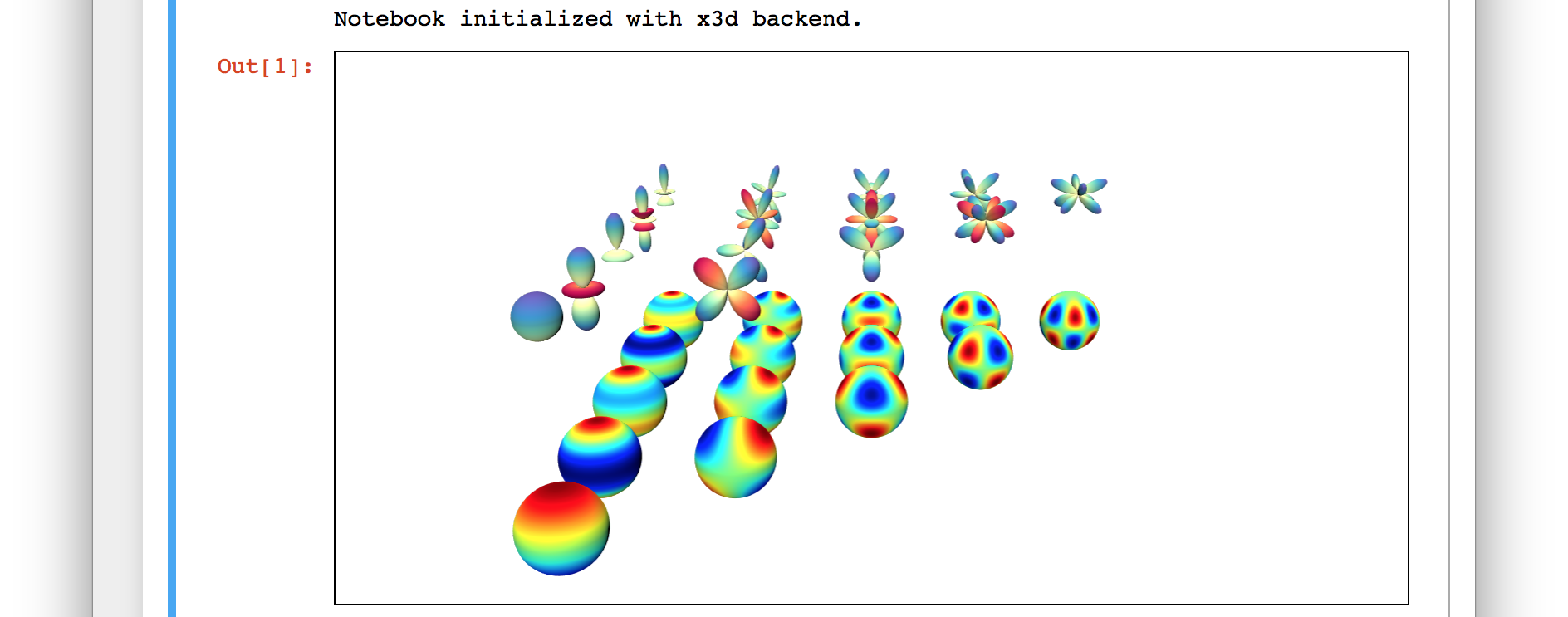
Inside the loop, `mlab.mesh` prints a Mayavi object, but Jupyter does not. When I tried to output the Mayavi object outside the loop, I saw a 3D object. ʻU` contains only the last created Mayavi object, but with a panoramic view. I feel that it would be good if there was an opportunity for 3D drawing.
# 3D display from other than Mayavi (during delusion)
Jupyter notebook with embedded 3D data is a very attractive data exchange format. I would be happy if it could be used by people other than Mayavi. I haven't established a method yet, but I would like to make two comments.
The first is a modification of the x3d format. When I open the Jupyter notebook (extension `.ipynb`) with a text editor, the data in x3d format is embedded. (3D objects represented by x3d are only lines and faces, so even a small scene will be long text)
```text
"outputs": [
{
"data": {
"text/html": [
"\n",
" <?xml version=\"1.0\" encoding =\"UTF-8\"?>\n",
"\n",
"<X3D profile=\"Immersive\" version=\"3.0\" id=\"scene_1\" >\n",
" <head>\n",
" <meta name=\"filename\" content=\"Stream\"/>\n",
" <meta name=\"generator\" content=\"Visualization ToolKit X3D exporter v0.9.1\"/>\n",
" <meta name=\"numberofelements\" content=\"1\"/>\n",
" </head>\n",
" <Scene>\n",
" <Background skyColor=\"0.5 0.5 0.5\"/>\n",
```
When I modified this x3d scene in an editor and reloaded it in Jupyter notebook, the 3D scene changed. So if you introduce the text in x3d format from another program, you should be able to view 3D images from other than Mayavi.
one more point. It would be convenient to draw a file in which Jupyter notebook is saved in HTML format in 3D even in an environment where Juopyter is not installed.
Now, the file Jupyter notebook saved in HTML format contains x3d data, but when I open it in a browser, 3D is not drawn. The part that instructs x3d drawing is here, but since it points to a local file, it probably was not drawn.
```html
<script type="text/javascript">
require(["/nbextensions/mayavi/x3d/x3dom.js"], function(x3dom) { /**/
var x3dom_css = document.getElementById("x3dom-css");
if (x3dom_css === null) {
var l = document.createElement("link");
l.setAttribute("rel", "stylesheet");
l.setAttribute("type", "text/css");
l.setAttribute("href", "/nbextensions/mayavi/x3d/x3dom.css"); /**/
l.setAttribute("id", "x3dom-css");
$("head").append(l);
}
if (typeof x3dom != 'undefined') {
x3dom.reload();
}
else if (typeof window.x3dom != 'undefined') {
window.x3dom.reload();
}
})
</script>
```
Rewrite the reference to the Mayavi plugin in nbextension to x3dom.org.
* Fixed `/nbextensions/mayavi/x3d/x3dom.js` to` http://www.x3dom.org/download/x3dom.js`
* Modified `/nbextensions/mayavi/x3d/x3dom.css` to` http://www.x3dom.org/download/x3dom.css`
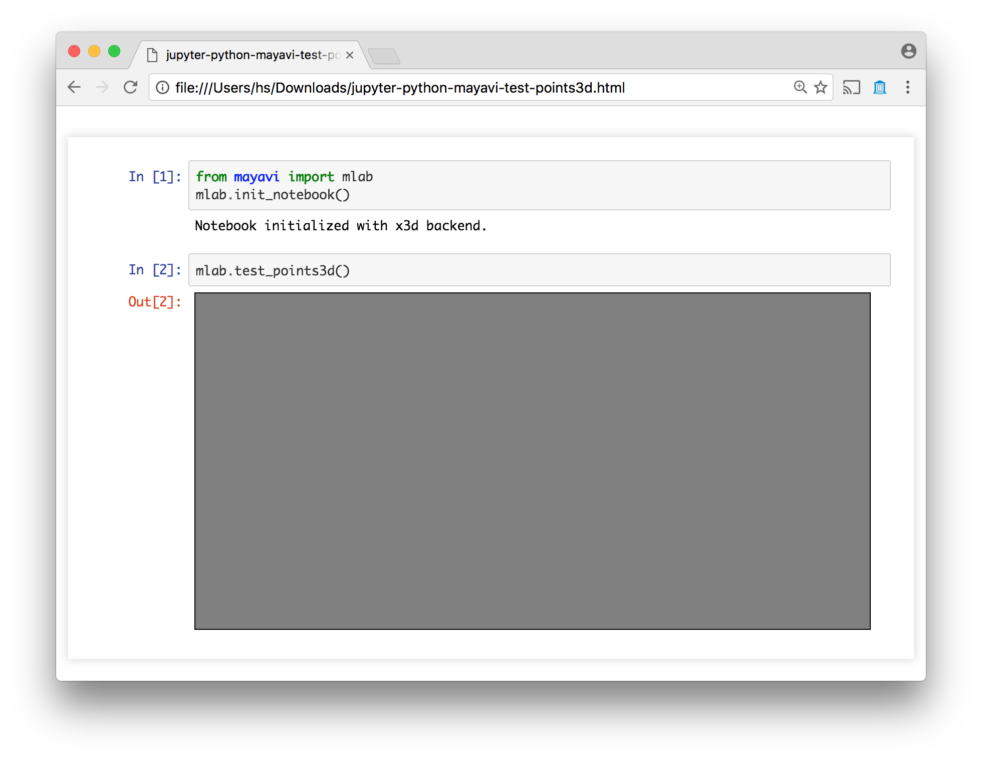
Then, the 3D drawing area was drawn, but the 3D object was not drawn yet.
Let's think about the above two points a little more. If it goes well, I would like to add it.
I'm sorry I ended up with a delusion at the end.
Recommended Posts