Drawing with Bezier curve and Fourier transform

This is the first post. I intend to write it so that even high school students can understand it. Please forgive that the implementation is difficult to read.

The characters in the picture are Suzu Kagura (green) and Yamatoiori (light blue) from .LIVE. The work on this page is a derivative work. Intellectual property rights related to characters belong to Upland Co., Ltd.

Work example

This is the one.

Rough flow

Make a collection of ordered dots that form a picture when tied ↓ Fast Fourier transform of x and y coordinates respectively ↓ Can be drawn by superposition of circular motion

environment

• macOS Big Sur 11.1
• PowerPoint for Mac 16.44
• Python 3.7.4
• beautifulsoup4 4.8.0
• matplotlib 3.1.1 (can be done without)
• numpy 1.17.2
• pillow 6.2.0
• tqdm 4.36.1 (can be done without)

procedure

If you already have a collection of points that will make a picture when connected, skip to the Discrete Fourier Transform.

Draw a picture in PowerPoint

In PowerPoint "Curve", write a picture __ one stroke __. Writing with one stroke is quite difficult.

Rewrite .pptx to .zip and unzip

If you rewrite .pptx to .zip and decompress it, the following xml will appear. I referred to I wish the normal distribution could be drawn in PowerPoint.

Unzipped file/ppt/slides/slide1.xml

(abridgement)
<a:pathLst>
    <a:path w="6982104" h="6267205">
        <a:moveTo>
            <a:pt x="2424619" y="3964459"/>
        </a:moveTo>
        <a:cubicBezTo>
            <a:pt x="2459747" y="3967701"/>
            <a:pt x="2494875" y="3970944"/>
            <a:pt x="2534866" y="3945004"/>
        </a:cubicBezTo>
        <a:cubicBezTo>
            <a:pt x="2574858" y="3919064"/>
            <a:pt x="2615930" y="3853132"/>
            <a:pt x="2664568" y="3808817"/>
        </a:cubicBezTo>
        <a:cubicBezTo>
            <a:pt x="2713206" y="3764502"/>
            <a:pt x="2757521" y="3720187"/>
            <a:pt x="2826695" y="3679115"/>
        </a:cubicBezTo>
        <a:cubicBezTo>
(abridgement)

Cubic Bézier curves are specified by four points. See "Cubic Bézier curves" in English wikipedia for more information. The meaning of the contents of xml

xml

(abridgement)
    <a:pt The first control point and the fourth control point on the previous curve/>
</a:cubicBezTo>
<a:cubicBezTo>
    <a:pt 2nd control point/>
    <a:pt 3rd control point/>
    <a:pt 4th control point and 1st control point on the curve after/>
</a:cubicBezTo>
(abridgement)

It seems that it looks like this.

Bezier curve implementation

Control points as $ P_ {0}, P_ {1}, P_ {2}, P_ {3} $ Bezier curve B(t) = (1-t)^{3}P_{0}+3(1-t)^{2}tP_{1}+3(1-t)t^{2}P_{2}+t^{3}P_{3},\quad 0\leq t\leq 1 Is expressed as. I implemented it as it is.

python

import numpy as np

class BezFunc:
    
    #p is a list of 4 control points
    def __init__(self, p):
        self.p0 = np.array(p[0])
        self.p1 = np.array(p[1])
        self.p2 = np.array(p[2])
        self.p3 = np.array(p[3])
        
    # 0<=t<=1
    def __call__(self, t):
        return ((1-t)**3)*self.p0+3*((1-t)**2)*t*self.p1+3*(1-t)*(t**2)*self.p2+(t**3)*self.p3

Extract control points from xml and draw a curve

Use BeautifulSoup to retrieve control points from xml.

python

from bs4 import BeautifulSoup
import numpy as np

    
class Points:
    
    def __init__(self, xml_path):
        with open(xml_path, 'r') as f:
            soup = BeautifulSoup(f, 'xml')

        # [[Control point 1,Control point 2,Control point 3,Control point 4], [Control point 1,Control point 2, …
        bez_points_list = []

        temp_pt = soup.find('a:pathLst').find('a:moveTo').find('a:pt')
        temp_point = (int(temp_pt['x']), int(temp_pt['y']))

        for temp_cubicBezTo in soup.find('a:pathLst').find_all('a:cubicBezTo'):
            temp_list = [temp_point]
            for temp_pt in temp_cubicBezTo.find_all('a:pt'):
                temp_point = (int(temp_pt['x']), int(temp_pt['y']))
                temp_list.append(temp_point)
            bez_points_list.append(temp_list)
        
        self.bez_points_list = bez_points_list

    # n :Division number
    def calc_points(self, n):
        points = []

        for bez_points in self.bez_points_list:
            f = BezFunc(bez_points)
            for i in range(n):
                t = i/n
                points.append(f(t))

        self.points = np.array(points)
        
    def get_points(self):
        return self.points

How to use

python

xml_path = 'presentation/ppt/slides/slide1.xml'
p = Points(xml_path)
p.calc_points(n=5) #5 divisions(suitable)
points = p.get_points()
points

array([[2424619.   , 3964459.   ], #Coordinates of the first point
       [2445734.704, 3966170.848], #Coordinates of the second point
       [2467083.832, 3966482.104], #Coordinates of the third point
       ...,
       [3557916.696, 5271117.176],
       [3503553.224, 5255947.584],
       [3548753.368, 5184643.528]])

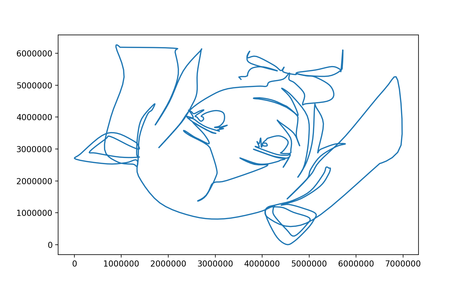
points is an array ofshape = (number of points, 2)numpy. If you connect these in order from the top, you can draw a picture.

python

import matplotlib.pyplot as plt

plt.figure(figsize=(8, 5), dpi=200)
plt.plot(points[:,0], points[:,1])
plt.show()

Discrete Fourier transform

Discrete Fourier transform and inverse transform

F(t) = \sum_{x=0}^{N-1}f(x)e^{-i\frac{2\pi t x}{N}}\\

f(x) = \frac{1}{N}\sum_{t=0}^{N-1}F(t)e^{i\frac{2\pi t x}{N}}

Then, when the discrete Fourier transform is performed and the inverse transform is performed, the original function is restored. Think of $ F (t) and \ quad f (x) $ as an array of N elements, respectively. this is,

Discrete Fourier transform

F(t) = \frac{1}{N}\sum_{x=0}^{N-1}f(x)e^{-i\frac{2\pi t x}{N}}\\

f(x) = \sum_{t=0}^{N-1}F(t)e^{i\frac{2\pi t x}{N}}

But the same is true.

here,

F(t) = A(t)( \cos \phi (t) + i \sin \phi (t))

Euler's formula

e^{i\theta}=\cos \theta + i \sin \theta

With, the inverse transformation

\begin{align}
f(x)&= \sum_{t=0}^{N-1}F(t)e^{i\frac{2\pi t x}{N}}\\
&= \sum_{t=0}^{N-1}A(t)( \cos \phi (t) + i \sin \phi (t))(\cos \frac{2\pi t x}{N} + i \sin \frac{2\pi t x}{N})\\
&= \sum_{t=0}^{N-1}A(t)(\cos (\phi (t) +\frac{2\pi t x}{N}) + i \sin (\phi (t) + \frac{2\pi t x}{N}))\\
&= \sum_{t=0}^{N-1}A(t)\cos (\phi (t) +\frac{2\pi t x}{N}) + i \sum_{t=0}^{N-1}A(t) \sin (\phi (t) + \frac{2\pi t x}{N})\\

\end{align}

And if $ f (x) $ is a real number, the second term will be zero, so

f(x)= \sum_{t=0}^{N-1}A(t)\cos (\phi (t) +\frac{2\pi t x}{N})

You can see that the inverse transformation can be represented by the projection of the superposition of circular motions onto a straight line.

Fast Fourier transform

Discrete Fourier transform formula

F(t) = \frac{1}{N}\sum_{x=0}^{N-1}f(x)e^{-i\frac{2\pi t x}{N}}

You can implement it as is, but using the Fast Fourier Transform (FFT) will result in a very short execution time. (Experience story)

numpy fft is

F(t) = \sum_{x=0}^{N-1}f(x)e^{-i\frac{2\pi t x}{N}}

Is designed to be calculated, so divide by N.

python

import numpy as np

F = np.fft.fft(One-dimensional array) / len(One-dimensional array)

This will give you a one-dimensional array of complex numbers.

F(t) = A(t)( \cos \phi (t) + i \sin \phi (t))

Because it was

A(t) = | F(t) |, \quad \phi(t) = \arg F(t)

You can calculate the amplitude and initial phase of the circular motion with.

python

import math

def complex_to_wave(F):
    results = []
    for i, temp_complex in enumerate(F):
        amp = abs(temp_complex) # A(t)Equivalent to
        freq = i #Equivalent to t
        phase = math.atan2(temp_complex.imag, temp_complex.real) # phi(t)Equivalent to
        results.append((amp, freq, phase))
    return sorted(results, reverse = True)

Diameter A (t) = amp Frequency t/N = freq/N Initial phase phi (t) = phase If you add up the circular motions of

f(x)= \sum_{t=0}^{N-1}A(t)\cos (\phi (t) +\frac{2\pi t x}{N})

You can reproduce the coordinate values.

Draw a picture with Pillow

With pillow, you can draw shapes with python. Please check the detailed usage.

That's what we're doing in the implementation below.

Subtract the average value of each from the one-dimensional array of x and y coordinates, and adjust the scale appropriately. ↓ Fast Fourier transform of each array is performed to obtain a one-dimensional array of complex numbers. ↓ From the complex number, calculate the amplitude, initial phase, and frequency of the overlapping circular motions. ↓ Draw in order from the circle with the largest amplitude.

python

import math
import numpy as np
from PIL import Image, ImageDraw
from tqdm import tqdm_notebook as tqdm

def draw(draw_info, save_name):

    original_points = np.array(draw_info['points'])

    epicycles_x = complex_to_wave(np.fft.fft(original_points[:,0])/len(original_points[:,0]))
    epicycles_y = complex_to_wave(np.fft.fft(original_points[:,1])/len(original_points[:,1]))

    width = 640
    height = 360
    center = (width // 2, height // 2)
    frames = len(epicycles_x)
    frame_interval = 5
    center_of_horizontal_circle = (400, 70)
    center_of_vertical_circle = (70, 200)

    images = []
    drawing_points = original_points + np.array([center_of_horizontal_circle[0],
                                                 center_of_vertical_circle[1]])

    for frame in tqdm(range(0, frames, frame_interval)):
        im = Image.new('RGB', (width, height), draw_info['background_color'])
        draw = ImageDraw.Draw(im)
        
        top_of_horizontal_circle = draw_epicycles(draw, epicycles_x, center_of_horizontal_circle,
                                                     frame, frames, vertical = False)
        top_of_vertical_circle = draw_epicycles(draw, epicycles_y, center_of_vertical_circle,
                                                   frame, frames, vertical = True)

        drawing_point = (top_of_horizontal_circle[0], top_of_vertical_circle[1])
        draw.line((top_of_horizontal_circle, drawing_point), fill = (0, 0, 0), width = 2)
        draw.line((top_of_vertical_circle, drawing_point), fill = (0, 0, 0), width = 2)
        draw_lines(draw, drawing_points[:frame], draw_info['colors'], draw_info['width'])
        
        images.append(im)

    images[0].save(f'{save_name}.gif',
                   save_all = True, append_images = images[1:],
                   optimizer = False, duration = 17, loop = 0)

def draw_lines(draw, drawing_points, drawing_colors, drawing_width):
    
    drawing_width = int(drawing_width)
    drawing_points = tuple([tuple(i) for i in drawing_points])
    length = len(drawing_points)
    
    for i in range(length - 1):
        
        draw.line((drawing_points[i], drawing_points[i + 1]),
                  fill = drawing_colors[i + 1], width = drawing_width)
        
def draw_epicycles(draw, epicycles, center_of_circle, frame, frames, vertical):
    
    if vertical:
        init_theta = math.pi / 2
    else:
        init_theta = 0
    
    for amp, freq, phase in epicycles:

        theta = 2*math.pi*freq*frame/frames + phase + init_theta
        center_of_next_circle = (center_of_circle[0] + amp * math.cos(theta),
                                 center_of_circle[1] + amp * math.sin(theta))

        draw.ellipse((center_of_circle[0] - amp, center_of_circle[1] - amp,
                      center_of_circle[0] + amp, center_of_circle[1] + amp),
                     outline = (127, 127, 127))
        draw.line((center_of_circle, center_of_next_circle),
                  fill = (127, 127, 127), width = 2)
        center_of_circle = center_of_next_circle
        
    return center_of_circle

python

draw_info = {'points' : (points - np.mean(points, axis=0))/13000,
             'width' : 3,
             'colors' : [(0, 190, 255) for _ in range(len(points))],
             'background_color' : (255, 255, 255)}
draw(draw_info, 'save_name')

Complete

GIF tends to have a large file size, so please convert it to mp4.

bonus

You can also do this.