[Python] My stock price forecast [HFT]
1. Motivation
- There are various articles about stock price forecasts even if you look at Qiita's article, but in this article I also decided to seriously try to forecast stock prices.
- The stock price forecast here is a ** short-term forecast ** that is a few minutes away.
- ** When you look at the board of the exchange, you may get the impression that buying is strong or selling is high, but this approach is to predict the stock price based on that.
- I referred to the paper "Deep Convolutional Neural Networks for Limit Order Books". Limit Order Book (LOB) means board information.
- In addition, the dataset uses data from the Helsinki Stock Exchange in Finland called FI-2010.
2. About board information
- For board information, the article Zai Online explains in an easy-to-understand manner. To put it simply, a board is a collection of the following selling and buying needs. Various people's buy and sell orders are gathered on the exchange. ●● Orders such as wanting to buy (sell) XX shares in yen are aggregated by price and the total number of shares is displayed.
| Selling quantity(ASK) | Stock price | Buy quantity(BID) |
|---|---|---|
| 500 | 670 | |
| 400 | 669 | |
| 600 | 668 | |
| 667 | 300 | |
| 666 | 1,200 | |
| 665 | 400 |
- There are various ways of thinking about why and how the stock price fluctuates, but here we think that if the selling quantity of the people who want to buy is larger than the selling quantity of the people who want to sell, the stock price will go up.
- In the example of the board above, consider the case where a person who wants to buy 100 shares appears and places a new order. There are roughly two patterns for ordering.
- The first method is to hit your own buy order even though there is a sell order for 600 shares for 668 yen. At this time, the board changes as shown below.
| ASK | Stock price | BID |
|---|---|---|
| 500 | 670 | |
| 400 | 669 | |
| 500 | 668 | |
| 667 | 300 | |
| 666 | 1,200 | |
| 665 | 400 |
- The other is to place a buy order for 667 yen, for example. It is not always executed, but the buy will be completed when a sell order comes out at 667 yen. At this time, the board changes as shown below.
| ASK | Stock price | BID |
|---|---|---|
| 500 | 670 | |
| 400 | 669 | |
| 600 | 668 | |
| 667 | 400 | |
| 666 | 1,200 | |
| 665 | 400 |
- What I want to say here is as follows.
- When the number of people who want to buy increases, the board information will be a reaction that ** the quantity of ASK decreases or the quantity of BID increases **.
- When the number of people who want to sell increases, the board information will be a reaction that ** the quantity of ASK increases or the quantity of BID decreases **.
- ** Do you feel that if you follow the board information carefully, you can get some suggestions about the stock price transition after that **? ??
3. FI-2010 dataset
What is the FI-2010 dataset?
- There is a detailed explanation in the paper Benchmark Dataset for Mid-Price Forecasting of Limit Order Book Data with Machine Learning Methods, and the following is an excerpt from it.
- Board information data taken from the Helsinki exchange in Finland.
- Data for the period from June 1st to 14th, 2010.
- The target stocks are 5 stocks. These are KESBV, Outokumpu (OUT1V), Sampo Concern (SAMPO), Rotorooky (RTRKS), and Wärtsilä (WET1V). I didn't know all the brands.
- It seems that the data is sampled every time there is a change in the board. (I feel that the number of data is small for that, so my understanding may be different here. However, I do not know because it is 2010.)
- You can download the normalized data. The following three types of normalization are available.
- Z-score
\quad x_i^{Zscore} = \frac{x_i - x_{mean}}{x_{std}} \quad \rm where \quad x_{mean} = \frac{1}{N} \sum_{j=1}^{N} x_j, \quad x_{std} = \sqrt{\frac{1}{N} \sum_{j=1}^{N} (x_j - x_{mean})^2} - Min-Max Scaling
\quad x_i^{(MM)} = \frac{x_i - x_{min}}{x_{max} - x_{min}} - Decimal Precision
\quad x_i^{DP} = \frac{x_i}{10^k} \quad where k is the integer that will give the maximum value for|x_i^{(DP)}|<1 - Click the Link here (https://etsin.avointiede.fi/dataset/urn-nbn-fi-csc-kata20170601153214969115) Data Availability Access this dataset freely. To download it.
Data overview
- Below we will look at the data normalized by Decimal Precision. This is because I think it is easiest to intuitively understand the numbers in the data. First of all, you can read the data of the first day out of all 10 days of data.
data = pd.read_csv('Train_Dst_Auction_DecPre_CF_1.txt',
                   header=None, delim_whitespace=True)
print(data.shape)
#=> (149, 47342)
- There are 47,342 data in total, and you can see that each is composed of 149 elements.
- It's hard to grasp the whole picture, so let's look at the heat map.
plt.figure(figsize=(20,10))
plt.imshow(data, interpolation='nearest', vmin=0, vmax=0.75,
           cmap='jet', aspect=data.shape[1]/data.shape[0])
plt.colorbar()
plt.grid(False)
plt.show()
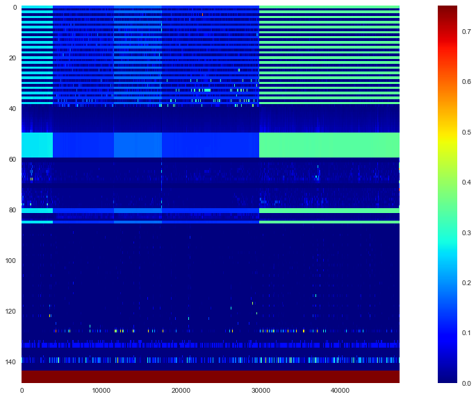
- If you look at this, you can see that the data of 5 brands are connected side by side. The 144 lines from the top represent features, and the last 5 lines represent labels. In addition, the paper has the following description about specific features.
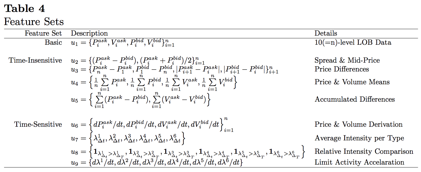
- Basic board information is in 40 lines of $ u_1 $. After that, the features are created by processing the board information. Let's take a closer look at how the data is contained in the board information. Use the first column as a test.
lob = data.iloc[:40,0].values
lob_df = pd.DataFrame(lob.reshape(10,4),
                      columns=['ask','ask_vol','bid','bid_vol'])
print(lob_df)
| ask | ask_vol | bid | bid_vol | |
|---|---|---|---|---|
| 0 | 0.2631 | 0.00392 | 0.2616 | 0.00663 |
| 1 | 0.2643 | 0.00028 | 0.2615 | 0.00500 |
| 2 | 0.2663 | 0.00165 | 0.2614 | 0.00500 |
| 3 | 0.2664 | 0.00500 | 0.2613 | 0.00043 |
| 4 | 0.2667 | 0.00039 | 0.2612 | 0.00646 |
| 5 | 0.2710 | 0.00700 | 0.2611 | 0.00200 |
| 6 | 0.2745 | 0.00200 | 0.2609 | 0.00199 |
| 7 | 0.2749 | 0.00487 | 0.2602 | 0.00081 |
| 8 | 0.2750 | 0.00300 | 0.2600 | 0.00197 |
| 9 | 0.2769 | 0.01000 | 0.2581 | 0.01321 |
- It's easy to understand when you come here. The best ASK and BID are at the top, and the board information is gradually becoming far from the best sign.
$ \ quad u_1 = \ {P_i ^ {ask}, V_i ^ {ask}, P_i ^ {bid}, V_i ^ {bid} \} _ {i = 1} ^ {10} $
As described in>, the data in 40 lines is in the form of "1st (best) ASK price, ASK quantity, BID price, BID quantity, 2nd ASK price, ASK quantity, BID price, BID quantity ..." It is stored in.
4. Model
Training data and labels
- From here, we will explain the machine learning model that is actually used. To learn, we need the training data $ \ mathbb X $ and the corresponding label $ \ mathbb y $, but it is about $ (\ mathbb x_t, y_t) $ that composes this.
- ** Data used for learning **, but at some point $ t $ board data
$ \ quad v_t = \ {P_ {t, i} ^ {ask}, V_ {t, i} ^ {ask}, P_ {t, i} ^ {bid}, V_ {t, i} ^ {bid} \} _ {i = 1} ^ {10} $
and this is the latest $ p One learning data ($ \ mathbb x \ _t $) is obtained by collecting $ pieces. Specifically,
$ \ quad \ mathbb x \ _t = \ begin {pmatrix} v \ _ {t-p + 1} \\ v \ _ {t-p + 2} \\ \ vdots \\ v \ _t \ end {pmatrix} = \ begin {pmatrix} P \ _ {t-p + 1,1} ^ {ask} & V \ _ {t-p + 1,1} ^ {ask} & P \ _ {t-p + 1,1} ^ {bid} & V \ _ {t-p + 1,1} ^ {bid} & P \ _ {t-p + 1,2} ^ {ask } & \ cdots & P \ _ {t-p + 1,10} ^ {bid} & V \ _ {t-p + 1,10} ^ {bid} \\ P \ _ {t-p + 2 , 1} ^ {ask} & V \ _ {t-p + 2,1} ^ {ask} & P \ _ {t-p + 2,1} ^ {bid} & V \ _ {t-p + 2,1} ^ {bid} & P \ _ {t-p + 2,2} ^ {ask} & \ cdots & P \ _ {t-p + 2,10} ^ {bid} & V \ _ { t-p + 2,10} ^ {bid} \\ \ vdots & \ vdots & \ vdots & \ vdots & \ vdots & \ ddots & \ vdots & \ vdots \\ P \ _ {t, 1} ^ {ask} & V \ _ {t, 1} ^ {ask} & P \ _ {t, 1} ^ {bid} & V \ _ {t, 1} ^ {bid} & P \ _ {t, 2 } ^ {ask} & \ cdots & P \ _ {t, 10} ^ {bid} & V \ _ {t, 10} ^ {bid} \ end {pmatrix} $
$ p × 40 $ It will be a queue. After convolving this with CNN, it is passed through LSTM, so the oldest data is in the first line, and the data at $ t $ is in the bottom line. - ** Label ** ($ y_t $) shows whether the average of the midpoints of the $ k $ period after $ t $ is rising, falling, or leveling off based on the threshold $ \ alpha
. Allocate to and. First, the midpoint ( p_t $) is the average of the best ASK and BID at each point in time, so
$ \ quad p_t = \ frac {P_ {t, 1} ^ {ask} + P_ { It becomes t, 1} ^ {bid}} {2} $
. Furthermore, the average value of the midpoint ($ m_ {+} (t)) and its rate of increase / decrease ( l_t $) in the period $ k $ are
$ \ quad m_ {+} (t) = \ frac. {1} {k} \ sum_ {i = 1} ^ {k} p_ {t + i}, \ quad l_t = \ frac {m_ {+} (t) --p_t} {p_t} $
can do. Finally, based on the threshold ($ \ alpha $),
$ \ quad y_t = \ left \ {\ begin {array} {} 1, & l_t> \ alpha \\ -1, & l_t < -\ alpha \\ 0, & \ rm otherwise \ end {array} \ right. $
Label it.
Model architecture
- The following is an example of the model first. First, the board information at each point in time is convoluted by CNN, and finally, the time series relationship is processed by LSTM.
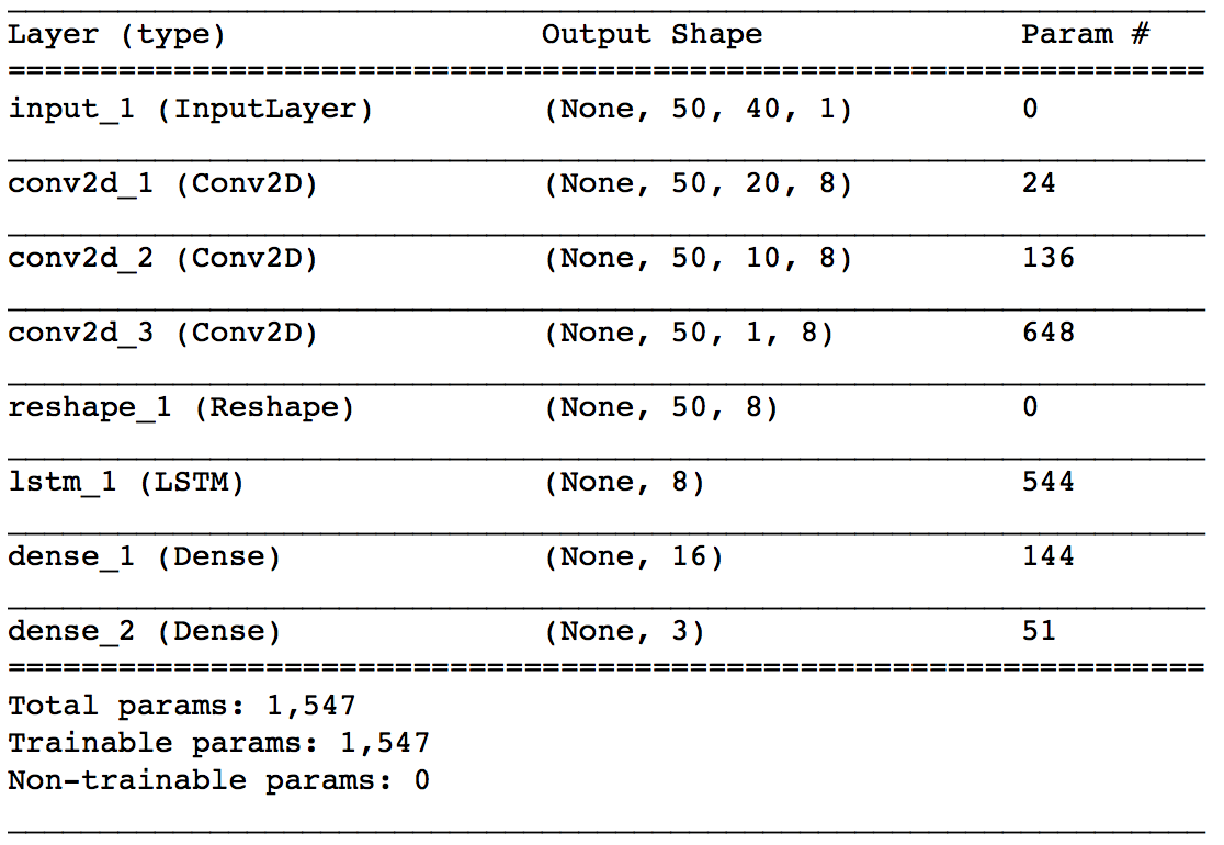
- ** input_1 ** Let's start with the layers. Output Shape means (batch size, number of board information to be referenced ($ p $), number of data included in one board information (40), 1). Here, $ p = 50 $.
- ** conv2d_1 ** The layer is the first convolution layer. The kernel size is $ 1 x 2 $ and the stride is $ 1 x 2 $. The price and quantity pairs of board information are listed in $ \ mathbb x_t $, but here we are convolving each pair. The number of kernels is specified as 8. Here, only the convolution in the row direction is performed, so the number of board information referenced by Output Shape remains unchanged at $ p (= 50) $, and the number of data contained in one board information is halved. I will.
The * ** conv2d_2 ** layer is also a convolution layer with a kernel size of $ 1x2 $ and a stride of $ 1x2
. The number of kernels is specified as 8. The convolution here is for the board information "ASK side price / quantity folded with conv2d_1" and "BID side price / quantity folded with conv2d_1", if the best sign About the best quote It plays the role of putting together the four numbers of ASK and BID price and quantity. Depending on the weight of conv2d_1 and conv2d_2, you can get a little image by thinking that it behaves like calculating the weighted average midpoint of the corresponding ASK and BID. This weighted average midpoint is also called the microprice ( p_t ^ {(micro)} $) and is defined as follows.
$ \ quad p_ {t, i} ^ {(micro)} = \ frac {P_ \ {t, i} ^ {ask} V_ \ {t, i} ^ {ask} + P_ \ {t, i} ^ {bid} V_ \ {t, i} ^ {bid}} {V_ \ {t, i} ^ {ask} + V_ \ {t, i} ^ {bid}} $ - ** The conv2d_3 ** layer is a convolution layer with a kernel size of $ 1 x 10 $ and a stride of $ 1 $. The number of kernels is specified as 8. In the first place, both sides of ASK and BID refer to 10 boards, so the output of conv2d_2 consists of 10 numbers for each board information. It is this layer that convolves these 10 numbers together. The board information at this point was folded into one number. The * ** reshape_1 ** layer is there to feed the output of conv2d_3 to the next lstm_1. The * ** ltsm_1 ** layer is trying to capture the time-series relationships of the board information that has been collapsed so far. The number of units specifies 8. The * ** dense_1 ** layer is a simple hidden layer that receives the output of the LSTM. The * ** dense_2 ** layer is the output layer for this network. Three outputs are used according to the number of label types, and softmax is used for activation.
5. Implementation
Data preprocessing
- Here, we will move the model using the data of the 5th brand with the largest number of samples among the data read earlier.
#Board information is in the first 40 lines. 29738 as the data of the fifth brand~Specify 47294.
lob = data.iloc[:40, 29738:47294].T.values
#Here, standardize by price and quantity.
lob = lob.reshape(-1,2)
lob = (lob - lob.mean(axis=0)) / lob.std(axis=0)
lob = lob.reshape(-1,40)
lob_df = pd.DataFrame(lob)
#Calculate the non-standardized midpoint.
lob_df['mid'] = (data.iloc[0,29738:47294].T.values + data.iloc[2,29738:47294].T.values) / 2
- When I plot the midpoint price, it looks like the following. Well, it's a common stock chart. There is an impression that there are many small vibrations because there are no limit prices for all bid prices that are close to the current price. The fact that stock prices are not data that keeps moving in one direction seems to be good for creating a model.

- Next, we will create a label.
#Specify the parameters.
p = 50
k = 50
alpha = 0.0003
#Create a label from the midpoint based on the parameters.
lob_df['lt'] = (lob_df['mid'].rolling(window=k).mean().shift(-k)-lob_df['mid'])/lob_df['mid']
lob_df = lob_df.dropna()
lob_df['label'] = 0
lob_df.loc[lob_df['lt']>alpha, 'label'] = 1
lob_df.loc[lob_df['lt']<-alpha, 'label'] = -1
-
The labeling by this parameter is as follows. When the stock price rises, it sends a rising signal, and when it falls, it sends a falling signal.

-
Load the required libraries.
from sklearn.model_selection import train_test_split
from keras.utils import to_categorical
from keras.layers import Conv2D, Dense, Reshape, Input, LSTM
from keras import Model, backend
import tensorflow as tf
- We will create learning data.
#Create training data.
X = np.zeros((len(lob_df)-p+1, p, 40, 1))
lob = lob_df.iloc[:,:40].values
for i in range(len(lob_df)-p+1):
    X[i] = lob[i:i+p,:].reshape(p,-1,1)
y = to_categorical(lob_df['label'].iloc[p-1:], 3)
print(X.shape, y.shape)
#=> (17457, 50, 40, 1) (17457, 3)
- Finally, it is divided into training data and test data.
X_train, X_test, y_train, y_test = train_test_split(X, y, test_size=0.2)
- This completes the pre-processing!
Model building
- From here, we will create a neural network model using keras. I'm more familiar with the Functional API than Sequential, so I'll write it here.
tf.reset_default_graph()
backend.clear_session()

inputs = Input(shape=(p,40,1))
x = Conv2D(8, kernel_size=(1,2), strides=(1,2), activation='relu')(inputs)
x = Conv2D(8, kernel_size=(1,2), strides=(1,2), activation='relu')(x)
x = Conv2D(8, kernel_size=(1,10), strides=1, activation='relu')(x)
x = Reshape((p, 8))(x)
x = LSTM(8, activation='relu')(x)
x = Dense(16, activation='relu')(x)
outputs = Dense(3, activation='softmax')(x)

model = Model(inputs=inputs, outputs=outputs)
model.compile(optimizer='adam', loss='categorical_crossentropy', metrics=['accuracy'])
Let's learn!
- All you have to do is learn.
epochs = 50
batch_size = 256
history = model.fit(X_train, y_train,
                    epochs=epochs,
                    batch_size=batch_size,
                    verbose=1,
                    validation_data=(X_test, y_test))
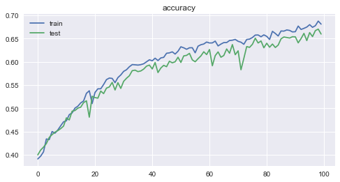
Epoch 100/100 13965/13965 [==============================] - 5s 326us/step - loss: 0.6526 - acc: 0.6808 - val_loss: 0.6984 - val_acc: 0.6595
- The loss and accuracy for each epoch are as follows. You can see how the learning is progressing reasonably well.

6. Consideration
-
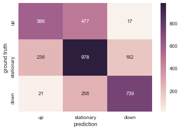
Accuracy was 0.6808 for training data, and 0.6595 ** for test data, which was an unexpectedly good result.
-
Let's visualize the result of the test data with a heat map. It is good that they can be classified correctly, but when considering practical use, "to give a down signal when the stock price rises" and "to give an up signal when the stock price falls" lead to loss. So it is the most problematic. In this regard, there are quite a few cases where the opposite signal is given, which is a positive result.
-
Future tasks
-
Hyperparameter tuning.
-
Learn data from other brands as well.
-
Learn using data from other trading days. (In general, it is known that even if a model is created based on the data of one day, the performance will deteriorate if it is used on another day.)
-
Verify if similar performance can be achieved in the recent Japanese stock market.
Recommended Posts