You can see it! Comparison of optimization methods (2020)
Target person
For those who want to see a comparison of each optimization method. Let's compare the methods introduced in here in various search spaces. If you have another good search plane or have a search space you would like to try, we are waiting for information.
table of contents
- x^2-y^2
- tanh(x)^2+tanh(y)^2
- -sin(x)/x-sin(y)/y+(x^2+y^2)/7 -[High-quality version](#High-quality version) -[Code used](# Code used)
x^2-y^2 For the time being
f(x, y) = x^2 - y^2
Let's search around the origin.
The initial position is $ (x_0, y_0) = (-1.5, -10 ^ {-4}) $. The $ y $ coordinates are not 0 because the learning rules include things that do not assume that the slope will be completely $ 0 $.
Well, it's okay to say that the gradient isn't completely $ 0 $.


 There are many learning rules that are not caught by the saddle point because there is a slight gradient in the $ y $ axis direction. The learning rules that are caught will eventually fall.
By the way, it looks like this when it is completely zero.
 Santa evaporates in an instant, and the learning rule, which does not matter if the gradient is completely zero, is completely captured by the saddle point. SMORMS3 no longer works with a jerk. There may be a mistake in the code ...
tanh(x)^2+tanh(y)^2 Next
f(x, y) = \tanh^2 x + \tanh^2 y
So, I tried it at the initial position $ (x, y) = (-1, 2) $.
After all, only SMORMS3 fits in the saddle point ...
Santa has gone somewhere, but you can see it coming back.


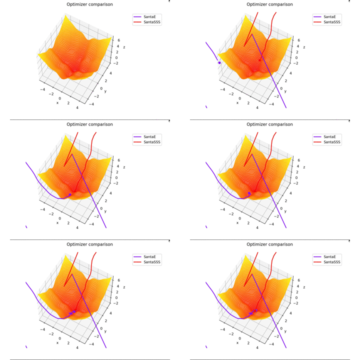
-sin(x)/x-sin(y)/y+(x^2+y^2)/7 continue
f(x, y) = -\cfrac{\sin (\pi x)}{\pi x} - \cfrac{\sin (\pi y)}{\pi y} + \cfrac{x^2+y^2}{7}
is. This is different from the others in $ x, y \ in [-5, 5] $, and the initial position is $ (x, y) = (-3, 4) $. $ \ Frac {x ^ 2 + y ^ 2} {7} $ is added to create a learning rule that fits the saddle point exquisitely and a learning rule that does not fit the saddle point.


 Regarding $ N $ in Santa's learning rule, as far as I read the dissertation, I felt that it was the number of mini-batch, so I set $ N = 1 $, but if $ N = 16 $, it will converge firmly. right...

By the way, it vibrates when $ N = epoch $.

I won't put it, but if you increase $ epoch $ and set $ N = epoch $, it will look like a coloring book lol
After all, it's okay to recognize that it is the number of mini-batch. Practically, $ N = 16,32 $, and at that value, it vibrates slightly.
Regarding $ N $ in Santa's learning rule, as far as I read the dissertation, I felt that it was the number of mini-batch, so I set $ N = 1 $, but if $ N = 16 $, it will converge firmly. right...

By the way, it vibrates when $ N = epoch $.

I won't put it, but if you increase $ epoch $ and set $ N = epoch $, it will look like a coloring book lol
After all, it's okay to recognize that it is the number of mini-batch. Practically, $ N = 16,32 $, and at that value, it vibrates slightly.
High quality version
The image quality is rougher than I expected, so I will leave a little high-quality version.
 The capacity limit that has been closed ...
Code used
Here is the experimental code. When I output the animation with jupyter notebook, the points and lines are displayed below the search plane and it is hard to see, so I am running it on the terminal.
Experimental code
test.py
#%matplotlib nbagg  #For jupyter
import numpy as np
import matplotlib.pyplot as plt
import matplotlib.animation as animation
from mpl_toolkits.mplot3d import Axes3D


from optimizers import *  #Comment out on jupyter
#It is assumed that the optimizers module is in the same folder.


def g(x, y):
    #return (x**2 - y**2) * 1
    #return np.tanh(x)**2 + np.tanh(y)**2
    return -(np.sinc(x) + np.sinc(y)) + (x**2 + y**2)/7


def dgx(x, y):
    #return 2*x * 1
    #return 2 * np.tanh(x) / np.cosh(x)**2
    return np.sin(np.pi*x)/(np.pi * x**2) + 2*x/7 - np.cos(np.pi*x)/x


def dgy(x, y):
    #return -2*y * 1
    #return 2 * np.tanh(y) / np.cosh(y)**2
    return np.sin(np.pi*y)/(np.pi * y**2) + 2*y/7 - np.cos(np.pi*y)/y


num = 401
#x = np.linspace(-2, 2, num)
#y = np.linspace(-2, 2, num)
x = np.linspace(-5, 5, num)
y = np.linspace(-5, 5, num)
X, Y = np.meshgrid(x, y)
Z = g(X, Y)
elevation = np.arange(np.min(Z), np.max(Z), 0.25)
#start_x = -1.5
#start_y = -1e-4
#start_x = -1
#start_y = 2
start_x = -3
start_y = 4
exact_x = 0
exact_y = 0
epoch = 500
N = epoch
seed=2
np.random.seed(seed=seed)
#fig = plt.figure()
#ax = fig.add_subplot(111, projection="3d")
#ax.set_zlim(-1, 1)
#im = ax.plot_surface(X, Y, Z, cmap="autumn")
#fig.show()

opt_dict = {
#    "SDG": SGD(eta=5e-2),
#    "MSGD": MSGD(eta=5e-2),
#    "NAG": NAG(eta=5e-2),
#    "AdaGrad": AdaGrad(eta=1e-1),
#    "RMSprop": RMSprop(eta=5e-2),
#    "AdaDelta": AdaDelta(),
#    "Adam": Adam(alpha=5e-2),
#    "RMSpropGraves": RMSpropGraves(eta=1e-2),
#    "SMORMS3": SMORMS3(eta=1e-2),
#    "AdaMax": AdaMax(alpha=2e-2),
#    "Nadam": Nadam(alpha=2e-2),
#    "Eve": Eve(alpha=5e-2),
    "SantaE": SantaE(eta=1e-3, burnin=10, N=N),
    "SantaSSS": SantaSSS(eta=1e-3, burnin=10, N=N),
#    "AMSGrad": AMSGrad(alpha=5e-2),
#    "AdaBound": AdaBound(alpha=5e-2),
#    "AMSBound": AMSBound(alpha=5e-2),
}
current_x = np.full(len(opt_dict), start_x, dtype=float)
current_y = np.full(len(opt_dict), start_y, dtype=float)

cmap = plt.get_cmap("rainbow")
coloring = [cmap(i) for i in np.linspace(0, 1, len(opt_dict))]

fig = plt.figure()
ax = fig.add_subplot(111, projection="3d")
ax.plot_surface(X, Y, Z, cmap="autumn", alpha=0.8)
ax.contour(X, Y, Z, cmap="autumn", levels=elevation, alpha=0.8)

ax.set_xlim(x[0], x[-1])
ax.set_ylim(y[0], y[-1])
ax.set_zlim(np.min(Z), np.max(Z))
ax.set_position([0.1, 0.1, 0.6, 0.8])
ax.set_xlabel("x")
ax.set_ylabel("y")
ax.set_zlabel("z")
ax.grid()
ax.view_init(60)


paths = np.zeros((epoch + 1, len(opt_dict), 3))
for j in range(len(opt_dict)):
    paths[0, j, 0] = current_x[j]
    paths[0, j, 1] = current_y[j]
    paths[0, j, 2] = g(current_x[j], current_y[j])
for i in range(1, epoch+1):
    for j, opt in enumerate(opt_dict):
        dx, dy = opt_dict[opt].update(dgx(current_x[j], current_y[j]),
                                      dgy(current_x[j], current_y[j]),
                                      t=i,
                                      w=current_x[j], b=current_y[j],
                                      dfw=dgx, dfb=dgy,
                                      f=g(current_x[j], current_y[j]))
        current_x[j] += dx
        current_y[j] += dy
        paths[i, j, 0] = current_x[j]
        paths[i, j, 1] = current_y[j]
        paths[i, j, 2] = g(current_x[j], current_y[j])


class TrajectoryAnimation3D(animation.FuncAnimation):
    def __init__(self, paths, labels=[], fig=None, ax=None, frames=None,
                 interval=60, repeat_delay=5, blit=True, coloring=None,
                 **kwargs):
        if fig is None:
            if ax is None:
                fig, ax = plt.subplots()
            else:
                fig = ax.get_figure()
        else:
            if ax is None:
                ax = fig.gca()

        self.fig = fig
        self.ax = ax
        self.paths = paths

        if frames is None:
            frames = paths.shape[0]

        self.lines = []
        self.points = []
        for j, opt in enumerate(labels):
            line, = ax.plot([], [], [], label=opt, lw=2, color=coloring[j])
            point, = ax.plot([], [], [], marker="o", color=coloring[j])
            self.lines.append(line)
            self.points.append(point)

        super().__init__(fig, self.animate, init_func=self.init_anim,
                         frames=frames, interval=interval, blit=blit,
                         repeat_delay=repeat_delay, **kwargs)

    def init_anim(self):
        for line, point in zip(self.lines, self.points):
            line.set_data([], [])
            line.set_3d_properties([])
            point.set_data([], [])
            point.set_3d_properties([])
        return self.lines + self.points

    def animate(self, i):
        j = int(0)
        for line, point in zip(self.lines, self.points):
            line.set_data(self.paths[:i, j, 0], self.paths[:i, j, 1])
            line.set_3d_properties(self.paths[:i, j, 2])
            point.set_data(self.paths[i, j, 0], self.paths[i, j, 1])
            point.set_3d_properties(self.paths[i, j, 2])
            j += 1
        return self.lines + self.points


anim = TrajectoryAnimation3D(paths, labels=opt_dict, fig=fig, ax=ax,
                             coloring=coloring)
fig.legend(bbox_to_anchor=(0.96, 0.9))
fig.suptitle("Optimizer comparison")
plt.show()
reference
-3D plot with matplotlib -Try rotating the 3D (3D) topographic map with the animation function of matplotlib
Deep learning series
-Introduction to Deep Learning ~ Basics ~ -Introduction to Deep Learning ~ Coding Preparation ~ -Introduction to Deep Learning ~ Forward Propagation ~ -Introduction to Deep Learning ~ Backpropagation ~ -List of activation functions (2020) -Gradient descent method list (2020) -See and understand! Comparison of optimization methods (2020) -Thorough understanding of im2col -Complete understanding of numpy.pad function
Recommended Posts