I tried to extract a line art from an image with Deep Learning

When I noticed, GW passed by in a blink of an eye. This year's GW walked around Tokyo (including some Saitama) with the whole family. I climbed the Sky Tree, but I didn't think there were so many people. It seemed interesting to go at night if I had to go next. It looks like it's being screened.

6/11 update

I modified the network structure and various things in the dataset to improve the line art that can be extracted, so I updated it including the contents.

I want a line art

As I wrote in the previous article, I tried line art coloring with Deep Learning, but in the process, I felt that there were some problems with the data set. The line art itself was created with reference to http://qiita.com/khsk/items/6cf4bae0166e4b12b942, but there seem to be some problems.

Binarizing a reduced image is too jagged
This itself was solved by binarizing and then shrinking (after all, shaggy appears when using BiCubic).
When using without binarization, depending on the color used, there are many cases where the originally darkened part becomes lighter.
Because the absolute value of the color difference is used, if similar colors are used between the line and the painted color, it will inevitably become lighter.
Depending on how the color is applied, extra details may appear.
Especially noticeable in shadows in anime painting

Well, there are some problems, but I am still working on it because it can be created easily (OpenCV should work) and at high speed (OpenCV is abbreviated).

Research to turn rough into line art

Some of the existing research is as follows. http://hi.cs.waseda.ac.jp:8081/

This is a dissertation. http://hi.cs.waseda.ac.jp/~esimo/publications/SimoSerraSIGGRAPH2016.pdf

This is a technique for AutoEncoder that converts rough to line art. This time, I made it with reference to this.

class AutoEncoder(object):
    """Define autoencoder"""

    def __init__(self):
        self.conv1 = Encoder(3, 48, 5, 5, strides=[1, 2, 2, 1], name='encoder1')
        self.conv1_f1 = Encoder(48, 128, 3, 3, name='encoder1_flat1')
        self.conv1_f2 = Encoder(128, 128, 3, 3, name='encoder1_flat2')
        self.conv2 = Encoder(128, 256, 5, 5, strides=[1, 2, 2, 1], name='encoder2')
        self.conv2_f1 = Encoder(256, 256, 3, 3, name='encoder2_flat1')
        self.conv2_f2 = Encoder(256, 256, 3, 3, name='encoder2_flat2')
        self.conv3 = Encoder(256, 256, 5, 5, strides=[1, 2, 2, 1], name='encoder3')
        self.conv3_f1 = Encoder(256, 512, 3, 3, name='encoder3_flat1')
        self.conv3_f2 = Encoder(512, 1024, 3, 3, name='encoder3_flat2')
        self.conv3_f3 = Encoder(1024, 512, 3, 3, name='encoder3_flat3')
        self.conv3_f4 = Encoder(512, 256, 3, 3, name='encoder3_flat4')

        self.bnc1 = op.BatchNormalization(name='bnc1')
        self.bnc1_f1 = op.BatchNormalization(name='bnc1_flat1')
        self.bnc1_f2 = op.BatchNormalization(name='bnc1_flat2')
        self.bnc2 = op.BatchNormalization(name='bnc2')
        self.bnc2_f1 = op.BatchNormalization(name='bnc2_flat1')
        self.bnc2_f2 = op.BatchNormalization(name='bnc2_flat2')
        self.bnc3 = op.BatchNormalization(name='bnc3')
        self.bnc3_f1 = op.BatchNormalization(name='bnc3_flat1')
        self.bnc3_f2 = op.BatchNormalization(name='bnc3_flat2')
        self.bnc3_f3 = op.BatchNormalization(name='bnc3_flat3')
        self.bnc3_f4 = op.BatchNormalization(name='bnc3_flat4')

        self.deconv1 = Decoder(256, 256, 4, 4, strides=[1, 2, 2, 1], name='decoder1')
        self.deconv1_f1 = Encoder(256, 128, 3, 3, name='decoder1_flat1')
        self.deconv1_f2 = Encoder(128, 128, 3, 3, name='decoder1_flat2')
        self.deconv2 = Decoder(128, 128, 4, 4, strides=[1, 2, 2, 1], name='decoder2')
        self.deconv2_f1 = Encoder(128, 128, 3, 3, name='decoder2_flat1')
        self.deconv2_f2 = Encoder(128, 48, 3, 3, name='decoder2_flat2')
        self.deconv3 = Decoder(48, 48, 4, 4, strides=[1, 2, 2, 1], name='decoder3')
        self.deconv3_f1 = Decoder(48, 24, 3, 3, name='decoder3_flat1')
        self.deconv3_f2 = Decoder(24, 1, 3, 3, name='decoder3_flat2')

        self.bnd1 = op.BatchNormalization(name='bnd1')
        self.bnd1_f1 = op.BatchNormalization(name='bnd1_flat1')
        self.bnd1_f2 = op.BatchNormalization(name='bnd1_flat2')
        self.bnd2 = op.BatchNormalization(name='bnd2')
        self.bnd2_f1 = op.BatchNormalization(name='bnd2_flat1')
        self.bnd2_f2 = op.BatchNormalization(name='bnd2_flat2')
        self.bnd3 = op.BatchNormalization(name='bnd3')
        self.bnd3_f1 = op.BatchNormalization(name='bnd3_flat1')


def autoencoder(images, height, width):
    """make autoencoder network"""

    AE = AutoEncoder()

    def div(v, d):
        return max(1, v // d)

    relu = tf.nn.relu
    net = relu(AE.bnc1(AE.conv1(images, [height, width])))
    net = relu(AE.bnc1_f1(AE.conv1_f1(net, [div(height, 2), div(width, 2)])))
    net = relu(AE.bnc1_f2(AE.conv1_f2(net, [div(height, 2), div(width, 2)])))
    net = relu(AE.bnc2(AE.conv2(net, [div(height, 2), div(width, 2)])))
    net = relu(AE.bnc2_f1(AE.conv2_f1(net, [div(height, 4), div(width, 4)])))
    net = relu(AE.bnc2_f2(AE.conv2_f2(net, [div(height, 4), div(width, 4)])))
    net = relu(AE.bnc3(AE.conv3(net, [div(height, 4), div(width, 4)])))
    net = relu(AE.bnc3_f1(AE.conv3_f1(net, [div(height, 8), div(width, 8)])))
    net = relu(AE.bnc3_f2(AE.conv3_f2(net, [div(height, 8), div(width, 8)])))
    net = relu(AE.bnc3_f3(AE.conv3_f3(net, [div(height, 8), div(width, 8)])))
    net = relu(AE.bnc3_f4(AE.conv3_f4(net, [div(height, 8), div(width, 8)])))
    net = relu(AE.bnd1(AE.deconv1(net, [div(height, 4), div(width, 4)])))
    net = relu(AE.bnd1_f1(AE.deconv1_f1(net, [div(height, 4), div(width, 4)])))
    net = relu(AE.bnd1_f2(AE.deconv1_f2(net, [div(height, 4), div(width, 4)])))
    net = relu(AE.bnd2(AE.deconv2(net, [div(height, 2), div(width, 2)])))
    net = relu(AE.bnd2_f1(AE.deconv2_f1(net, [div(height, 2), div(width, 2)])))
    net = relu(AE.bnd2_f2(AE.deconv2_f2(net, [div(height, 2), div(width, 2)])))
    net = relu(AE.bnd3(AE.deconv3(net, [height, width])))
    net = relu(AE.bnd3_f1(AE.deconv3_f1(net, [height, width])))

    net = tf.nn.sigmoid(AE.deconv3_f2(net, [height, width]))

    return net

AutoEncoder looks like this. I wondered if I could get it somehow. In the paper, it seems that the focus is on the method called loss map, but because I don't know how to refer to the histogram in Tensorflow, that part is implemented.

I tried it

The network used was about 250,000 times with the following parameters given.

batch size = 15
Patch size of learning image = 128 \ * 128
Randomly crop 128 \ * 128 from the original image and use
Randomly convert up / down / left / right / hue
learning rate = 0.00002
Optimizer = ADAM

I gave up on the huge size because I couldn't survive even with 2GiB memory in the first place. It seems good to reduce it once, extract it, and then insert an encoder to increase the resolution.

Image of reasonable size

Mikon! I painted it. Amezuku @ Looking for a job

All the original images are borrowed because I painted them with Pixiv. This image has no original line art, and there is no comparison target in the first place, so that's it. It took about 10 seconds for both this size and GPU, so I honestly don't want to think about doing it with a CPU.

I think it's pretty solid. The average size of the images in the dataset is about 1000 \ * 1000, which is quite large, so even large images can be handled. However, unfortunately there is a jaggedness peculiar to the lower part ... This can not be said because there are times when it comes out and times when it does not come out.

Thumbnail size

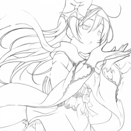
The size is 256 \ * 256. For the time being, I will also include the version I pulled out with OpenCV. Ignore the tsukkomi that 256 \ * 256 is thumbnailed.

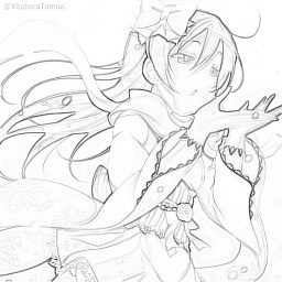
Original picture. At first glance, it seems like a line will appear, but ...

OpenCV version. Since all the fine color tones have come out, I can't deny the feeling that it's a line art or grayscale.

This network version. It's partly suspicious (or rather, the hand part is impossible to play), but the influence of the shadow can be ignored quite properly, and the expression of the hair part is simple, so it's a miso in the foreground, but it feels pretty good. Is it not? Too fine details such as frills are crushed by the stone, but it seems that this can be solved little by little if you continue learning a little more.

About dataset

The dataset used for learning is basically obtained from the categories painted by Pixiv. The most important thing in making a data set was that ** the line art and the colored image had the same aspect **. If this shifts, it will be like not being able to learn in the first place, so I collected them while checking each one.

Also, I sometimes found that even if the aspect ratio was the same, there was a slight difference between the line art and the colored image **. I had to omit it properly because learning would not proceed if there was this too.

Weaknesses

It depends on how you paint it, but it's a simpler line than OpenCV, and I think it feels like the details aren't lost that much. However, due to the structure or the nature of what we are doing, there are drawbacks, including the fact that there is nothing we can do about it.

The black part appears as it is
In the data used for learning, the black part remains as it is in a considerable proportion, coupled with the fact that the original line art itself was painted black.
Small size tends to blur
This is because the original image was at least 256 \ * 256 in size, so I feel that it is not possible to handle when more detailed features are met.
Basically give up on blurred parts
I also tried to force it to learn with a faint image with a Gaussian filter, but it is quite tight.
The part painted with almost the same color as the line color becomes quite ambiguous
Depends on dark shadows and painting method
It is basically impossible to reproduce the original (something is added on the line)

Basically, rather than using it as it is, I think it will be more like processing based on this.

Summary

Generating networks such as AutoEncoder are interesting. I also want to challenge myself to give parameters and change the way line art is made.

It is difficult to investigate and implement, but since amateurs can do deep learning, we recommend that you invest a little and try it (on your own or in the cloud).