100 Language Processing Knock 2020 Chapter 7: Word Vector

The other day, 100 Language Processing Knock 2020 was released. I myself have only been in natural language processing for a year, and I don't know the details, but I will solve all the problems and publish them in order to improve my technical skills.

All shall be executed on jupyter notebook, and the restrictions of the problem statement may be broken conveniently. The source code is also on github. Yes.

Chapter 6 is here.

The environment is Python 3.8.2 and Ubuntu 18.04.

Chapter 7: Word Vector

Create a program that performs the following processing for a word vector (word embedding) that expresses the meaning of a word as a real vector.

Please download the required dataset from here.

The downloaded file shall be placed under data.

60. Reading and displaying word vectors

Download the learned word vector (3 million words / phrases, 300 dimensions) in the Google News dataset (about 100 billion words) and display the word vector of "United States". However, note that "United States" is internally referred to as "United_States".

Use gensim.

code

from gensim.models import KeyedVectors

code

model = KeyedVectors.load_word2vec_format('data/GoogleNews-vectors-negative300.bin.gz', binary=True)

code

model["United_States"]

output

array([-3.61328125e-02, -4.83398438e-02,  2.35351562e-01,  1.74804688e-01,
       -1.46484375e-01, -7.42187500e-02, -1.01562500e-01, -7.71484375e-02,
        1.09375000e-01, -5.71289062e-02, -1.48437500e-01, -6.00585938e-02,
        1.74804688e-01, -7.71484375e-02,  2.58789062e-02, -7.66601562e-02,
       -3.80859375e-02,  1.35742188e-01,  3.75976562e-02, -4.19921875e-02,
       -3.56445312e-02,  5.34667969e-02,  3.68118286e-04, -1.66992188e-01,
       -1.17187500e-01,  1.41601562e-01, -1.69921875e-01, -6.49414062e-02,
       -1.66992188e-01,  1.00585938e-01,  1.15722656e-01, -2.18750000e-01,
       -9.86328125e-02, -2.56347656e-02,  1.23046875e-01, -3.54003906e-02,
       -1.58203125e-01, -1.60156250e-01,  2.94189453e-02,  8.15429688e-02,
        6.88476562e-02,  1.87500000e-01,  6.49414062e-02,  1.15234375e-01,
       -2.27050781e-02,  3.32031250e-01, -3.27148438e-02,  1.77734375e-01,
       -2.08007812e-01,  4.54101562e-02, -1.23901367e-02,  1.19628906e-01,
        7.44628906e-03, -9.03320312e-03,  1.14257812e-01,  1.69921875e-01,
       -2.38281250e-01, -2.79541016e-02, -1.21093750e-01,  2.47802734e-02,
        7.71484375e-02, -2.81982422e-02, -4.71191406e-02,  1.78222656e-02,
       -1.23046875e-01, -5.32226562e-02,  2.68554688e-02, -3.11279297e-02,
       -5.59082031e-02, -5.00488281e-02, -3.73535156e-02,  1.25976562e-01,
        5.61523438e-02,  1.51367188e-01,  4.29687500e-02, -2.08007812e-01,
       -4.78515625e-02,  2.78320312e-02,  1.81640625e-01,  2.20703125e-01,
       -3.61328125e-02, -8.39843750e-02, -3.69548798e-05, -9.52148438e-02,
       -1.25000000e-01, -1.95312500e-01, -1.50390625e-01, -4.15039062e-02,
        1.31835938e-01,  1.17675781e-01,  1.91650391e-02,  5.51757812e-02,
       -9.42382812e-02, -1.08886719e-01,  7.32421875e-02, -1.15234375e-01,
        8.93554688e-02, -1.40625000e-01,  1.45507812e-01,  4.49218750e-02,
       -1.10473633e-02, -1.62353516e-02,  4.05883789e-03,  3.75976562e-02,
       -6.98242188e-02, -5.46875000e-02,  2.17285156e-02, -9.47265625e-02,
        4.24804688e-02,  1.81884766e-02, -1.73339844e-02,  4.63867188e-02,
       -1.42578125e-01,  1.99218750e-01,  1.10839844e-01,  2.58789062e-02,
       -7.08007812e-02, -5.54199219e-02,  3.45703125e-01,  1.61132812e-01,
       -2.44140625e-01, -2.59765625e-01, -9.71679688e-02,  8.00781250e-02,
       -8.78906250e-02, -7.22656250e-02,  1.42578125e-01, -8.54492188e-02,
       -3.18359375e-01,  8.30078125e-02,  6.34765625e-02,  1.64062500e-01,
       -1.92382812e-01, -1.17675781e-01, -5.41992188e-02, -1.56250000e-01,
       -1.21582031e-01, -4.95605469e-02,  1.20117188e-01, -3.83300781e-02,
        5.51757812e-02, -8.97216797e-03,  4.32128906e-02,  6.93359375e-02,
        8.93554688e-02,  2.53906250e-01,  1.65039062e-01,  1.64062500e-01,
       -1.41601562e-01,  4.58984375e-02,  1.97265625e-01, -8.98437500e-02,
        3.90625000e-02, -1.51367188e-01, -8.60595703e-03, -1.17675781e-01,
       -1.97265625e-01, -1.12792969e-01,  1.29882812e-01,  1.96289062e-01,
        1.56402588e-03,  3.93066406e-02,  2.17773438e-01, -1.43554688e-01,
        6.03027344e-02, -1.35742188e-01,  1.16210938e-01, -1.59912109e-02,
        2.79296875e-01,  1.46484375e-01, -1.19628906e-01,  1.76757812e-01,
        1.28906250e-01, -1.49414062e-01,  6.93359375e-02, -1.72851562e-01,
        9.22851562e-02,  1.33056641e-02, -2.00195312e-01, -9.76562500e-02,
       -1.65039062e-01, -2.46093750e-01, -2.35595703e-02, -2.11914062e-01,
        1.84570312e-01, -1.85546875e-02,  2.16796875e-01,  5.05371094e-02,
        2.02636719e-02,  4.25781250e-01,  1.28906250e-01, -2.77099609e-02,
        1.29882812e-01, -1.15722656e-01, -2.05078125e-02,  1.49414062e-01,
        7.81250000e-03, -2.05078125e-01, -8.05664062e-02, -2.67578125e-01,
       -2.29492188e-02, -8.20312500e-02,  8.64257812e-02,  7.61718750e-02,
       -3.66210938e-02,  5.22460938e-02, -1.22070312e-01, -1.44042969e-02,
       -2.69531250e-01,  8.44726562e-02, -2.52685547e-02, -2.96630859e-02,
       -1.68945312e-01,  1.93359375e-01, -1.08398438e-01,  1.94091797e-02,
       -1.80664062e-01,  1.93359375e-01, -7.08007812e-02,  5.85937500e-02,
       -1.01562500e-01, -1.31835938e-01,  7.51953125e-02, -7.66601562e-02,
        3.37219238e-03, -8.59375000e-02,  1.25000000e-01,  2.92968750e-02,
        1.70898438e-01, -9.37500000e-02, -1.09375000e-01, -2.50244141e-02,
        2.11914062e-01, -4.44335938e-02,  6.12792969e-02,  2.62451172e-02,
       -1.77734375e-01,  1.23046875e-01, -7.42187500e-02, -1.67968750e-01,
       -1.08886719e-01, -9.04083252e-04, -7.37304688e-02,  5.49316406e-02,
        6.03027344e-02,  8.39843750e-02,  9.17968750e-02, -1.32812500e-01,
        1.22070312e-01, -8.78906250e-03,  1.19140625e-01, -1.94335938e-01,
       -6.64062500e-02, -2.07031250e-01,  7.37304688e-02,  8.93554688e-02,
        1.81884766e-02, -1.20605469e-01, -2.61230469e-02,  2.67333984e-02,
        7.76367188e-02, -8.30078125e-02,  6.78710938e-02, -3.54003906e-02,
        3.10546875e-01, -2.42919922e-02, -1.41601562e-01, -2.08007812e-01,
       -4.57763672e-03, -6.54296875e-02, -4.95605469e-02,  2.22656250e-01,
        1.53320312e-01, -1.38671875e-01, -5.24902344e-02,  4.24804688e-02,
       -2.38281250e-01,  1.56250000e-01,  5.83648682e-04, -1.20605469e-01,
       -9.22851562e-02, -4.44335938e-02,  3.61328125e-02, -1.86767578e-02,
       -8.25195312e-02, -8.25195312e-02, -4.05273438e-02,  1.19018555e-02,
        1.69921875e-01, -2.80761719e-02,  3.03649902e-03,  9.32617188e-02,
       -8.49609375e-02,  1.57470703e-02,  7.03125000e-02,  1.62353516e-02,
       -2.27050781e-02,  3.51562500e-02,  2.47070312e-01, -2.67333984e-02],
      dtype=float32)

61. Word similarity

Calculate the cosine similarity between "United States" and "U.S.".

code

model.similarity("United_States", "U.S.")

output

0.73107743

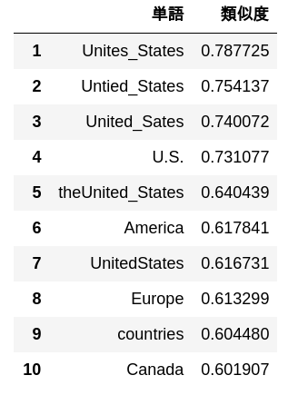
62. 10 words with high similarity

Output 10 words with high cosine similarity to “United States” and their similarity.

code

import numpy as np
import pandas as pd

code

simularities = model.most_similar("United_States")
pd.DataFrame(
    simularities,
    columns = ['word', 'Degree of similarity'],
    index = np.arange(len(simularities)) + 1
)

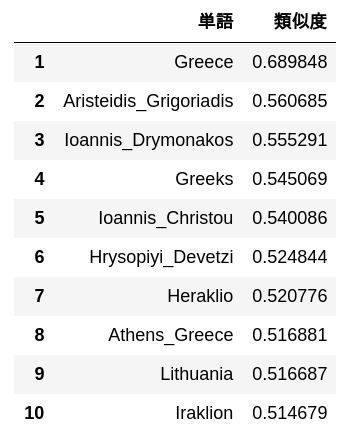
63. Analogy by additive construct

Subtract the "Madrid" vector from the "Spain" word vector, calculate the vector by adding the "Athens" vector, and output 10 words with high similarity to that vector and their similarity.

code

simularities = model.most_similar(positive=['Spain', 'Athens'], negative=['Madrid'])
pd.DataFrame(
    simularities,
    columns = ['word', 'Degree of similarity'],
    index = np.arange(len(simularities)) + 1
)

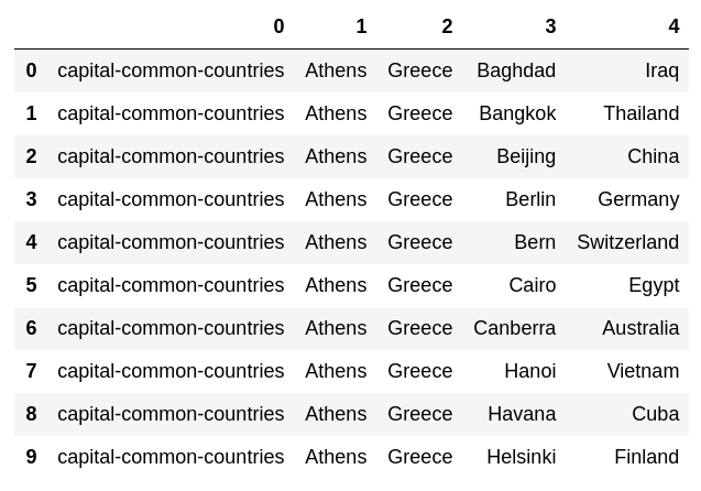
64. Experiments with analogy data

Download the evaluation data of the word analogy, calculate vec (word in the second column) --vec (word in the first column) + vec (word in the third column), and find the word with the highest similarity to the vector. ， Find the similarity. Add the obtained word and similarity to the end of each case.

code

with open('data/questions-words.txt') as f:
    lines = f.read().splitlines()

dataset = []
category = None
for line in lines:
    if line.startswith(':'):
        category = line[2:]
    else:
        lst = [category] + line.split(' ')
        dataset.append(lst)

code

pd.DataFrame(dataset[:10])

code

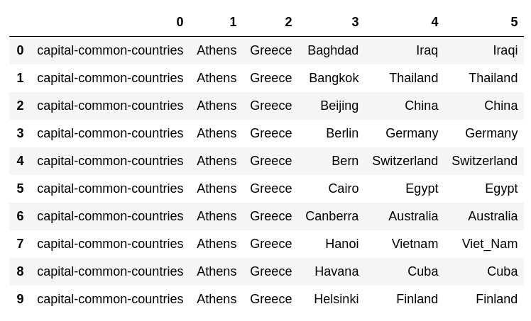
from tqdm import tqdm

code

for i, lst in enumerate(tqdm(dataset)):
    pred, prob = model.most_similar(positive = lst[2:4], negative = lst[1:2], topn = 1)[0]
    dataset[i].append(pred)

code

pd.DataFrame(dataset[:10])

65. Correct answer rate in analogy tasks

Measure the accuracy rate of the semantic analogy and the syntactic analogy using the execution results of> 64.

The theory that evaluate_word_analogies () should be used is widely known.

code

semantic_analogy = [lst[-2:] for lst in dataset if not lst[0].startswith('gram')]
syntactic_analogy = [lst[-2:] for lst in dataset if lst[0].startswith('gram')]

code

acc = np.mean([true == pred for true, pred in semantic_analogy])
print('Semantic analogy correct answer rate:', acc)

output

Semantic analogy correct answer rate: 0.7308602999210734

code

acc = np.mean([true == pred for true, pred in syntactic_analogy])
print('Literary analogy correct answer rate:', acc)

output

Literary analogy correct answer rate: 0.7400468384074942

66. Evaluation by WordSimilarity-353

Download the evaluation data of The WordSimilarity-353 Test Collection and calculate the Spearman correlation coefficient between the ranking of similarity calculated by the word vector and the ranking of human similarity judgment.

code

import zipfile

code

#Read from zip file
with zipfile.ZipFile('data/wordsim353.zip') as f:
    with f.open('combined.csv') as g:
        data = g.read()

#Decode byte sequence
data = data.decode('UTF-8').splitlines()
data = data[1:]

#Tab delimited
data = [line.split(',') for line in data]
len(data)

output

353

code

for i, lst in enumerate(data):
    sim = model.similarity(lst[0], lst[1])
    data[i].append(sim)

code

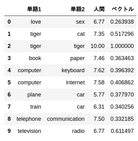
pd.DataFrame(
    data[:10],
    columns = ['Word 1', 'Word 2', 'Human', 'vector']
)

code

from scipy.stats import spearmanr

It is possible to apply argsort twice to get the ranking, but it may be useless in terms of calculation amount.

code

def rank(x):
    args = np.argsort(-np.array(x))
    rank = np.empty_like(args)
    rank[args] = np.arange(len(x))
    return rank

code

human = [float(lst[2]) for lst in data]
w2v = [lst[3] for lst in data]
human_rank = rank(human)
w2v_rank = rank(w2v)
rho, p_value = spearmanr(human_rank, w2v_rank)

output

Rank correlation coefficient: 0.700313895424209
p-value: 2.4846350292113526e-53

code

print('Rank correlation coefficient:', rho)
print('p-value:', p_value)

code

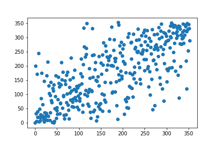
import matplotlib.pyplot as plt

code

plt.scatter(human_rank, w2v_rank)
plt.show()

67. k-means clustering

Extract the word vector related to the country name and execute k-means clustering with the number of clusters k = 5.

I'm not sure where to get the country name from, but the analogy dataset does a good job

code

countries = {
    country
    for lst in dataset
    for country in [lst[2], lst[4]]
    if lst[0] in {'capital-common-countries', 'capital-world'}
} | {
    country
    for lst in dataset
    for country in [lst[1], lst[3]]
    if lst[0] in {'currency', 'gram6-nationality-adjective'}
}
countries = list(countries)
len(countries)

output

129

code

country_vectors = [model[country] for country in countries]

code

from sklearn.cluster import KMeans

code

kmeans = KMeans(n_clusters=5)
kmeans.fit(country_vectors)

output

KMeans(algorithm='auto', copy_x=True, init='k-means++', max_iter=300,
       n_clusters=5, n_init=10, n_jobs=None, precompute_distances='auto',
       random_state=None, tol=0.0001, verbose=0)

code

for i in range(5):
    cluster = np.where(kmeans.labels_ == i)[0]
    print('class', i)
    print(', '.join([countries[k] for k in cluster]))

output

Class 0
Suriname, Honduras, Tuvalu, Guyana, Venezuela, Peru, Cuba, Ecuador, Nicaragua, Dominica, Colombia, Belize, Mexico, Bahamas, Jamaica, Chile
Class 1
Netherlands, Egypt, France, Syria, Finland, Germany, Uruguay, Switzerland, Greenland, Italy, Lebanon, Malta, Algeria, Europe, Tunisia, Brazil, Ireland, England, Libya, Spain, Argentina, Liechtenstein, Iran, Jordan, USA, Iceland, Sweden, Norway, Qatar, Portugal, Denmark, Canada, Israel, Belgium, Morocco, Austria
Class 2
Kazakhstan, Lithuania, Turkmenistan, Serbia, Croatia, Greece, Uzbekistan, Armenia, Latvia, Albania, Slovenia, Cyprus, Ukraine, Georgia, Belarus, Bulgaria, Kyrgyzstan, Macedonia, Estonia, Montenegro, Turkey, Azerbaijan, Tajikistan, Poland, Russia, Romania, Hungary, Slovakia, Moldova
Class 3
Ghana, Senegal, Zambia, Sudan, Somalia, Zimbabwe, Gabon, Madagascar, Angola, Liberia, Gambia, Niger, Uganda, Mauritania, Namibia, Eritrea, Botswana, Malawi, Mozambique, Guinea, Kenya, Nigeria, Burundi, Mali, Rwanda
Class 4
Japan, China, Pakistan, Samoa, Bahrain, Fiji, Australia, India, Laos, Bhutan, Malaysia, Taiwan, Cambodia, Nepal, Korea, Oman, Thailand, Bangladesh, Indonesia, Iraq, Vietnam, Afghanistan, Philippines

They are divided.

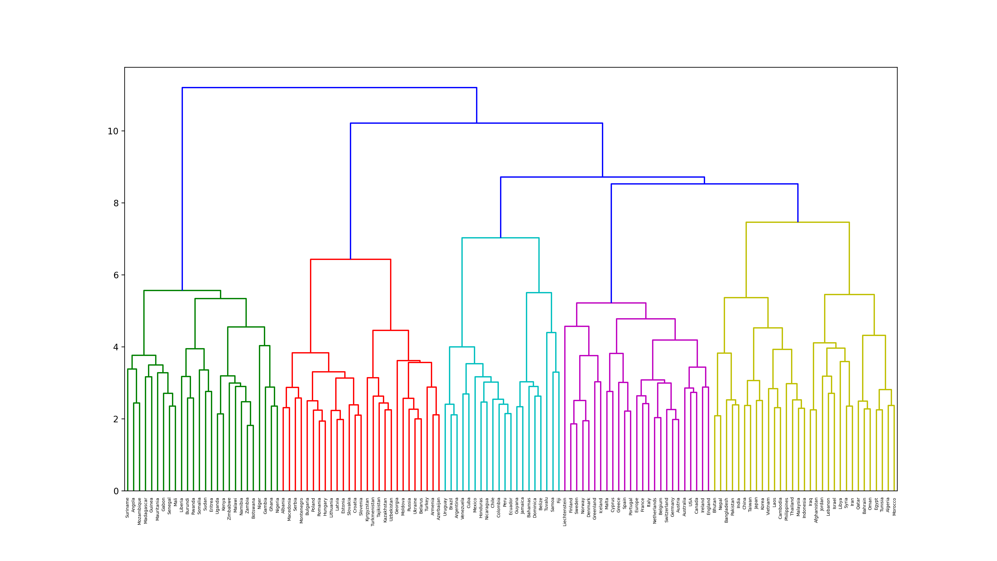
68. Ward's method clustering

Execute hierarchical clustering by Ward's method for word vectors related to country names. Furthermore, visualize the clustering result as a dendrogram.

code

from scipy.cluster.hierarchy import dendrogram, linkage

code

plt.figure(figsize=(16, 9), dpi=200)
Z = linkage(country_vectors, method='ward')
dendrogram(Z, labels = countries)
plt.show()

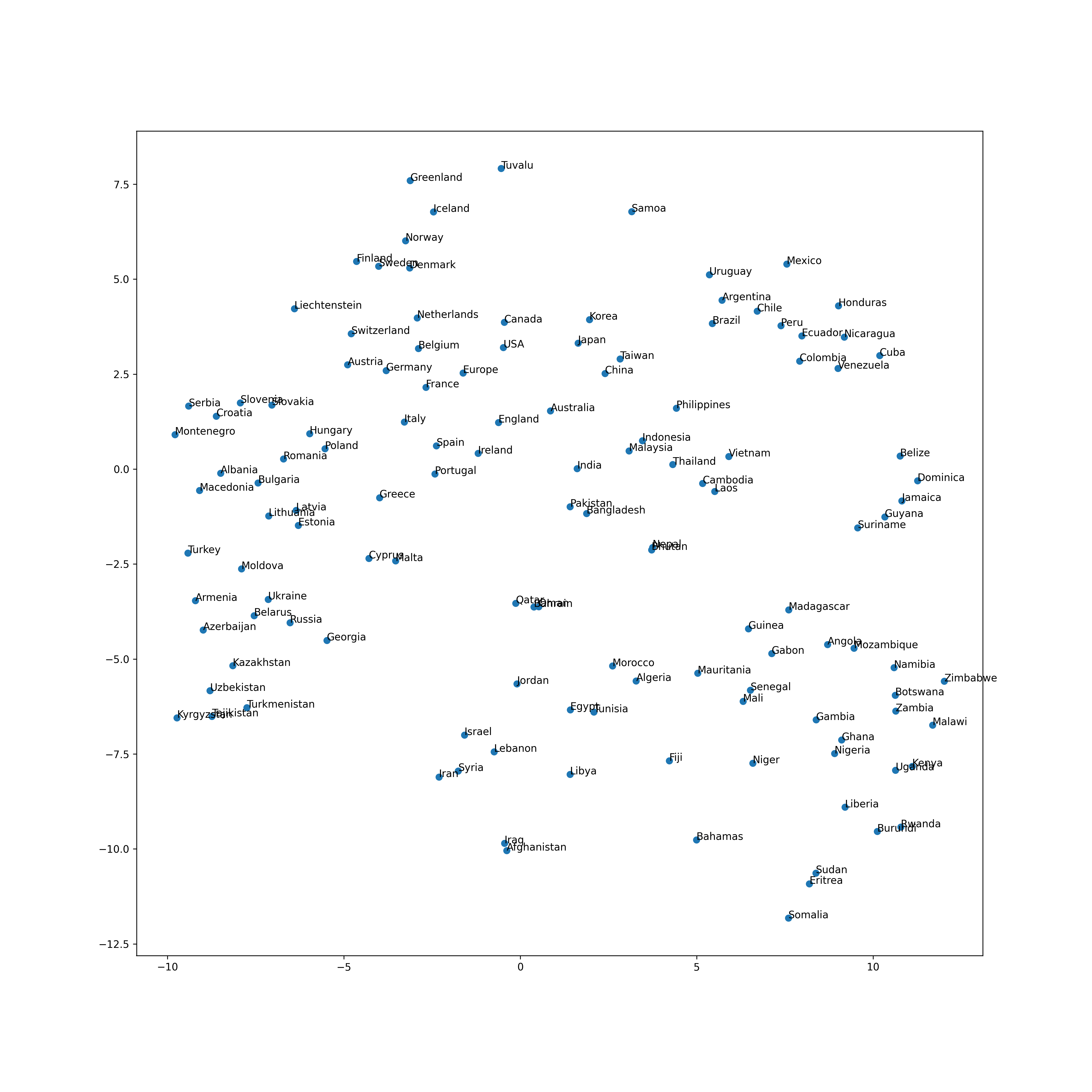
69. Visualization by t-SNE

Visualize the vector space of word vectors related to country names with t-SNE.

code

from sklearn.manifold import TSNE

code

tsne = TSNE()
tsne.fit(country_vectors)

output

TSNE(angle=0.5, early_exaggeration=12.0, init='random', learning_rate=200.0,
     method='barnes_hut', metric='euclidean', min_grad_norm=1e-07,
     n_components=2, n_iter=1000, n_iter_without_progress=300, n_jobs=None,
     perplexity=30.0, random_state=None, verbose=0)

code

plt.figure(figsize=(15, 15), dpi=300)
plt.scatter(tsne.embedding_[:, 0], tsne.embedding_[:, 1])
for (x, y), name in zip(tsne.embedding_, countries):
    plt.annotate(name, (x, y))
plt.show()

Next is Chapter 8

Language processing 100 knocks 2020 Chapter 8: Neural network