[Machine learning] What is the LP norm?

When studying machine learning, I think the terms L1 regularization and L2 regularization come up. [^ 1]

[^ 1]: TJO's "Blog of Data Scientists Working in Ginza" Practice L1 / L2 regularization in R Is also taken up.

Penalty term for L1 regularization: The L1 norm looks like this,

Penalty term for L2 regularization: The L2 norm looks like this,

Let's dig a little deeper into why the L1 norm and L2 norm are represented in this way.

Definition of Lp norm

Vector $ {\ bf x} $ in n dimensions,

{\bf x} = (x_1, \cdots, x_n)

Then the $ L ^ p $ norm is defined as follows.

\| {\bf x} \|_p = (\ |x_1|^p + |x_2|^p + \cdots + |x_n|^p )^{1/p}

L1 norm

Here, the $ L ^ 1 $ norm when $ {\ bf x} $ is two-dimensional so that it can be drawn in the graph is

\| {\bf x} \|_1 = |x_1| + |x_2|

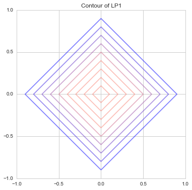
It is just the addition of the absolute values of $ x_1 $ and $ x_2 $. What is represented by contour lines That's how it was. This is also called [Manhattan distance](https://ja.wikipedia.org/wiki/Manhattan distance), and since there are only vertical and horizontal vertical roads like a grid, only vertical or horizontal movement is possible, and it moves diagonally. It is the same as the one that represents the distance of the world that you cannot do it. In other words, the light blue, red, and green lines are all 10 in length like this, so if you connect the same distance with a line, it will be a straight line like this. So the contour lines in the graph above are diamond-shaped, aren't they?

L2 norm

Similarly, the $ L ^ 2 $ norm of a two-dimensional vector is

\| {\bf x} \|_2 = \sqrt{|x_1|^2 + |x_2|^2}

is. This is the familiar Euclidean distance. Since the distance from the origin of the point on the circumference is always constant, it becomes a contour line that draws a beautiful circle as shown below.

Norms at various ps

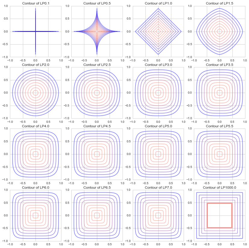
The L1 and L2 norms are often used in machine learning, but for the sake of understanding, I tried to see what contour lines are drawn with various p values.

I drew a diagram of $ p = 1000 $, with $ 0.5 $ each from $ p = 0.1, \ p = 0.5 to 7.5 $. (Originally, $ p $ in the Lp norm is a real number in $ p \ ge1 $, but I dared to draw 0.1 and 0.5.)

It turns out that when p approaches 0, it becomes a shape like "+", when it approaches 1, it becomes a diamond shape (a square rotated by 45 degrees), when it approaches 2, it becomes a circle, and when it approaches ∞, it becomes a shape like "□". I will.

(Although it is outside the definition of Lp norm, if there is a world with p = 0.1, it is a very difficult world to go diagonally: sweat_smile :)

These L1 and L2 norms are applied and used in Lasso regression, Ridge regression, ElasticNet, etc .: kissing_closed_eyes:

Python code @GitHub

The code for the main part of this article is below.

def LP(x, y, lp=1):
    x = np.abs(x) 
    y = np.abs(y)
    return (x**lp + y**lp)**(1./lp)

def draw_lp_contour(lp=1, xlim=(0, 1), ylim=(0, 1)):
    n = 201
    X, Y = np.meshgrid(np.linspace(xlim[0], xlim[1], n), np.linspace(ylim[0], ylim[1], n))
    Z = LP(X, Y, lp) 
    cm = generate_cmap(['salmon', 'salmon', 'salmon', 'salmon', 'blue'])
    interval = [i/10. -1 for i in range(20)]
    
    plt.contour(X, Y, Z, interval, alpha=0.5, cmap=cm)
    plt.title("Contour of LP{}".format(lp))
    plt.xlim(xlim[0], xlim[1])
    plt.ylim(ylim[0], ylim[1])

#Draw a graph of 16 types of p values
fig =plt.figure(figsize=(14,14))
size = 4
for i, lp in enumerate(np.r_[[0.1], np.linspace(0.5, 7, 14), [1000]]):
    plt.subplot(size, size, i+1)
    draw_lp_contour(lp, (-1, 1),(-1, 1))

The full text of the Python code that drew this graph can be found on GitHub. https://github.com/matsuken92/Qiita_Contents/blob/master/General/LP-Norm.ipynb

reference

Wikipedia Lp space https://ja.wikipedia.org/wiki/Lp空間

Online Machine Learning (Machine Learning Professional Series) [Umino, Okanohara, Tokui, Tokunaga] 　http://www.kspub.co.jp/book/detail/1529038.html

Practice L1 / L2 regularization with R 　http://tjo.hatenablog.com/entry/2015/03/03/190000

Effect of L1 regularization and L2 regularization on regression model 　http://breakbee.hatenablog.jp/entry/2015/03/08/041411