Matrix Convolution Filtering-Reinventor of Python Image Processing-
A story about convolution filtering only by matrix operation without relying on the image processing library. Also possible with Pythonista
** Click here for basics **
What is a "reinventor"?
Instead of relying on Open CV or Pillow, I will actually write various image processing using numpy and matplotlib. It's a combination that can also be used with the iOS app Pythonista.
import numpy as np
import matplotlib.pyplot as plt
In addition, the following functions are convenient for displaying images. (For details, Basics)
def img_show(img : np.ndarray, cmap = 'gray', vmin = 0, vmax = 255, interpolation = 'none') -> None:
    '''np.Display an image with array as an argument.'''

    #Set dtype to uint8
    img = np.clip(img,vmin,vmax).astype(np.uint8)

    #Display image
    plt.imshow(img, cmap = cmap, vmin = vmin, vmax = vmax, interpolation = interpolation)
    plt.show()
    plt.close()
Filtering by convolution
Spatial filtering is easy to understand for the filter by convolution.
First, create a function to convolve a two-dimensional array.
def convolve2d(img, kernel):
    #Calculate the size of the submatrix
    sub_shape = tuple(np.subtract(img.shape, kernel.shape) + 1)

    #Since the function name is long, it is omitted once
    strd = np.lib.stride_tricks.as_strided

    #Create a matrix of submatrix
    submatrices = strd(img,kernel.shape + sub_shape,img.strides * 2)

    #Calculate the Einstein sum of the submatrix and the kernel
    convolved_matrix = np.einsum('ij,ijkl->kl', kernel, submatrices)

    return convolved_matrix
The above code convolves using the matrix of the img submatrix. See stackoverflow teacher for more information. In this algorithm, the peripheral part can be removed.
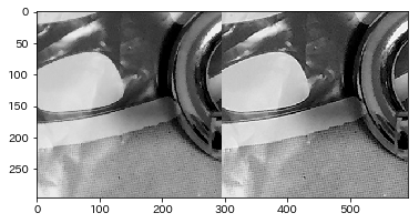
[Trimming]'tiger.jpeg'(http://qiita.com/secang0/items/1229212a37d8c9922901#%E5%9B%9B%E8%A7%92% E5% BD% A2% E3% 81% AB% E3% 83% 88% E3% 83% AA% E3% 83% 9F% E3% 83% B3% E3% 82% B0330% E8% BF% BD% E5% 8A% A0) image [weighted averaging by NTSC coefficient](http://qiita.com/secang0/items/6fba02d7cc3ef34c0c31#ntsc-%E4%BF%82%E6%95%B0%E3%81%AB % E3% 82% 88% E3% 82% 8B% E5% 8A% A0% E9% 87% 8D% E5% B9% B3% E5% 9D% 87% E6% B3% 95) for grayscale images On the other hand, various filters were used.
img = plt.imread('tiger.jpeg')[1200:1500,1400:1700]
img = (0.298912 * img[...,0] + 0.586611 * img[...,1] + 0.114478 * img[...,2])
img_show(img)

Low pass filter
A low-pass filter is a filter that tends to leave a low frequency part rather than a high frequency part of an image. (High / low is frequency) In short, it blurs by making the sudden changes less. This process is often used for noise removal.
img_show(convolve2d(img, kernel))
In the table below, concatenate is used to line up with the original image.
| Method name | Kernel / original image / filter image | Remarks |
|---|---|---|
| Simple moving average filter | kernel = np.ones((5,5)/25  |
The simplest low pass filter |
| Gaussian filter | kernel = gaussian_kernel(5)  |
Excellent low-pass filter based on normal distribution |
In the original image, the light gray part (yellowish green in the color image) in the center is stippled. However, applying a low-pass filter makes confirmation difficult.
In the table, the following Gaussian matrix is used. Reference
def gaussian_kernel(n : int) -> np.ndarray:
    '''(n,n)Make a Gaussian matrix of'''

    #[nC0, nC1, ..., nCn]Create
    combs = [1]
    for i in range(1,n):
        ratio = (n-i)/(i)
        combs.append(combs[-1]*ratio)
    combs = np.array(combs).reshape(1,n)/(2**(n-1))

    #Make a Gaussian matrix by the product of vertical and horizontal vectors
    result = combs.T.dot(combs)
    return result
High pass filter
A high-pass filter is a filter that tends to leave a high frequency part rather than a low frequency part of an image. As a result, the various parts are emphasized and the image becomes sharp.
A typical sharpening filter is for $ k> 0 $
1.\hspace{5pt}
\left(
\begin{matrix}
0&-k&0\\
-k&1+4k&-k\\
0&-k&0\\
\end{matrix}
\right)
\\
\mbox{Or}
\\
2.\hspace{5pt}

\left(
\begin{matrix}
-k&-k&-k\\
-k&1+8k&-k\\
-k&-k&-k\\
\end{matrix}
\right)
sharp_kernel_1 = lambda k : np.matrix('0,{0},0;{0},{1},{0};0,{0},0'.format(-k,1+4*k))
sharp_kernel_2 = lambda k : np.matrix('{0},{0},{0};{0},{1},{0};{0},{0},{0}'.format(-k,1+8*k))
Call. Reference The larger the value of k, the stronger the filter. Also, if k is the same, 2 is stronger.
The image is 3 * 3 Gaussian filtered, and the display is standardized as described below.
img_gaussian = convolve2d(img, gaussian(3))
img_show(norm_img(convolve2d(img_gaussian, kernel)))
In the table below, concatenate is used to line up with the original image. The light gray part below (yellowish green in a color image) is originally stippled and has many high frequency components. Please pay particular attention.
| Kernel / original image / filter image |
|---|
kernel = sharp_kernel_1(1) |
kernel = sharp_kernel_1(10) |
kernel = sharp_kernel_1(1) |
kernel = sharp_kernel_2(10) |
Since the pixel value of the filter image does not fit in 0 to 255, it is standardized by the following function. This corresponds the interval of $ mean \ pm n_ {std} \ times standard deviation $ to 0 ~ 255. (Actually $ n_ {std} = 2 $) This is a process that is also used for the original image for comparison, and is slightly different from the top image.
def norm_img(img_filtered,n_std):
    '''img_Standardize filtered'''
    mean = img_filtered.mean() #average
    std = img_filtered.std() #standard deviation
    img_norm = 256*((img_filtered - mean)/std + n_std)/(n_std*2)
    return np.clip(img_norm,0,255).astype(np.uint8)
differential
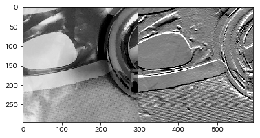
Derivative filters are used for contour extraction. This is because by finding the difference from the adjacent pixel, you can see where the change is large.
reference: ** Actual results are displayed ** ** Explains various differences between filters **.
The image is 3 * 3 Gaussian filtered. In addition, [High-pass filter section](http://qiita.com/secang0/items/f3a3ff629988dc660d87#%E3%83%8F%E3%82%A4%E3%83%91%E3%82%B9 % E3% 83% 95% E3% 82% A3% E3% 83% AB% E3% 82% BF% E3% 83% BC) The standardization process described in) was applied.
img_gaussian = convolve2d(img, gaussian(3))
img_show(norm_img(convolve2d(img_gaussian, kernel)))
| Contents | Kernel / original image / filter image | Remarks | Reference link |
|---|---|---|---|
| Simple first derivative filter from bottom to top | kernel = np.matrix('0,-1,0;0,1,0;0,0,0') |
Sensitivetonoise | Withexplanation |
| Prewitt filter from bottom to top | kernel = np.matrix('-1,-1,-1;0,0,0;1,1,1') |
Withresultimage&Withexplanation | |
| Sobel filter from bottom to top | kernel = np.matrix('-1,-2,-1;0,0,0;1,2,1') |
np.matrix('-1,-1,-1;0,0,0;1,1,1')*1.33Thedifferencewith |
Withresultimage&Withexplanation |
| Laplacian filter | kernel = np.matrix('-1,-1,-1;-1,8,-1;-1,-1,-1') |
Secondderivativeinalldirections |
Withresultimage&Withexplanation |
Other
| Contents | Kernel / original image / filter image | Remarks | Reference link |
|---|---|---|---|
| Embossing | kernel = np.matrix('-2,-1,0;-1,1,1;0,1,2') |
1inthecenterofSobel | Resultimageatthebottom |
Recommended Posts