What is magnetohydrodynamics?

Fluid dynamics that handle highly electrically conductive fluids such as plasma and liquid metals are called ** Magnetohydrodynamics **. It is often abbreviated from English as ** MHD **. The equation system of this magnetohydrodynamic is as follows when written in the conservative form.

\frac{\partial\mathbf{U}}{\partial t} + \frac{\partial\mathbf{F}}{\partial x} + \frac{\partial\mathbf{G}}{\partial y} + \frac{\partial\mathbf{H}}{\partial z}= \mathbf{0}

\mathbf{U} = \begin{bmatrix}
\rho \\
\rho u \\
\rho v \\
\rho w \\
B_x \\
B_y \\
B_z \\
e
\end{bmatrix},\ 
\mathbf{F} = \begin{bmatrix}
\rho u \\
\rho u^2+p_T-B_x^2 \\
\rho uv-B_xB_y \\
\rho uw-B_xB_z \\
0 \\
B_yu-B_xv \\
B_zu-B_xw \\
\left(e+p_T\right)u-B_x\left(\mathbf{v}\cdot\mathbf{B}\right)
\end{bmatrix},\ 
\mathbf{G} = \begin{bmatrix}
\rho v \\
\rho vu-B_yB_x \\
\rho v^2+p_T-B_y^2 \\
\rho vw-B_yB_z \\
B_xv-B_yu \\
0 \\
B_zv-B_yw \\
\left(e+p_T\right)v-B_y\left(\mathbf{v}\cdot\mathbf{B}\right)
\end{bmatrix},\ 
\mathbf{H} = \begin{bmatrix}
\rho w \\
\rho wu-B_zB_x \\
\rho wv-B_zB_y \\
\rho w^2+p_T-B_z^2 \\
B_xw-B_zu \\
B_yw-B_zv \\
0 \\
\left(e+p_T\right)w-B_z\left(\mathbf{v}\cdot\mathbf{B}\right)
\end{bmatrix}

p = \left(\gamma-1\right)\left(e-\frac{1}{2}\rho|\mathbf{v}|^2-\frac{1}{2}|\mathbf{B}|^2\right),\ p_T = p+\frac{1}{2}|\mathbf{B}|^2

Where $ \ rho and p $ are the densities and pressures, $ u, v and w $ are the velocities in the $ x, y and z $ directions, respectively, and $ B_x, B_y and B_z $ are $ x, y and z $ respectively. The magnetic field in the direction, and $ e $ represents the energy density. $ \ Gamma $ is the heat capacity ratio. Also, here, a unit system such as $ \ mu_0, 4 \ pi $ where the coefficients related to the magnetic field disappear is adopted. If you compare it with a normal fluid, you can see that a magnetic field is newly added as a variable.

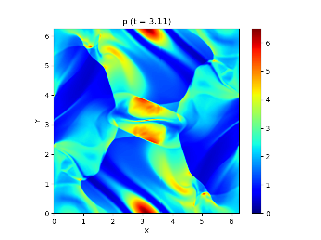
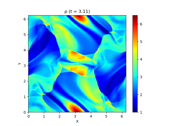
Now, a well-known problem with this magnetohydrodynamic is the ** Orszag-Tang vortex problem ** (Orszag and Tang, 1979) (Google Image Search). It is known that intricately entwined patterns are formed while vortices form shock waves, and if the magnetic field divergence generated numerically cannot be properly removed, the calculation is likely to fail, and this is a standard test for magnetic fluid calculation. It is often used as a problem. The specific settings are as follows.

\rho = \gamma^2,\ p = \gamma

u = -\sin y,\ v = \sin x,\ w = 0

B_x = -\sin y,\ B_y = \sin 2x,\ B_z = 0

\gamma = 5/3,\ 0\le x \le 2\pi,\ 0\le y \le 2\pi

Boundary conditions impose periodic boundary conditions in each of the $ x and y $ directions. This time the goal is to solve this. In the end, this figure is completed.

HLLD approximate Lehman solution

Here, for the sake of simplicity, let's make it one-dimensional. At this time, the equation system can be written as follows.

\frac{\partial\mathbf{U}}{\partial t} + \frac{\partial\mathbf{F}}{\partial x} = \mathbf{0}

\mathbf{U} = \begin{bmatrix}
\rho \\
\rho u \\
\rho v \\
\rho w \\
B_y \\
B_z \\
e
\end{bmatrix},\ 
\mathbf{F} = \begin{bmatrix}
\rho u \\
\rho u^2+p_T-B_x^2 \\
\rho uv-B_xB_y \\
\rho uw-B_xB_z \\
B_yu-B_xv \\
B_zu-B_xw \\
\left(e+p_T\right)u-B_x\left(\mathbf{v}\cdot\mathbf{B}\right)
\end{bmatrix}

For one dimension Maxwell's equations

\nabla\cdot\mathbf{B} = 0

Since $ B_x $ is always constant in time and space, $ B_x $ is excluded from the independent variable of the equation.

Now, by finding the Jacobian eigenvalues of $ \ mathbf {F} $ above, this magnetohydrodynamic has seven characteristic velocities.

\lambda_1 = u-c_{fx}, \lambda_2 = u-c_{ax}, \lambda_3 = u-c_{sx}, \lambda_4 = u, \lambda_5 = u+c_{sx}, \lambda_6 = u+c_{ax},\lambda_7 = u+c_{fx}

You can see that there is (I will omit it because derivation is insanely troublesome). here

a = \sqrt{\frac{\gamma p}{\rho}},\ c_{a} = \frac{|\mathbf{B}|}{\sqrt{\rho}}

c_{ax} = \frac{|B_x|}{\sqrt{\rho}},\ c_{fx,sx} = \left[\frac{a^2+c_a^2\pm\sqrt{\left(a^2+c_a^2\right)^2-4a^2c_{ax}^2}}{2}\right]^{1/2}

So, $ \ lambda_2, \ lambda_6 $ are ** Alfvén waves **, $ \ lambda_1, \ lambda_7 $ are ** fast magnetosonic waves **, $ \ lambda_3, \ lambda_5 $ are ** slow The slow magnetosonic wave ** and $ \ lambda_4 $ represent the ** entropy wave **. Considering that the normal fluid was a total of three types of sound waves before and after and entropy waves, the types of waves have increased considerably. Hmmm this looks hard. After all, it is 5 even without the slow-advancing magnetic sound wave, which is often ignored. Accurately capturing and calculating these wide variety of waves is considerably more difficult than with ordinary fluids.

Under such circumstances, ** HLLD approximate Lehman solution ** (Miyoshi and Kusano, 2005) is widely used as a solution with excellent accuracy, calculation efficiency, and robustness, and I would like to adopt this method this time.

Here, consider the following initial value problem that is discontinuously arranged with the origin as the boundary.

\mathbf{U} = \begin{cases}
\mathbf{U}_L & (x < 0) \\
\mathbf{U}_R & (x > 0)
\end{cases}

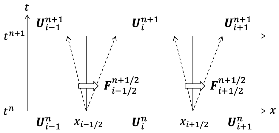
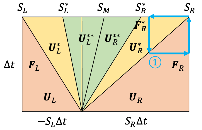
This is called the ** Lehman problem **, and in the scheme of the approximate Lehman solution system such as the HLLD method, $ \ mathbf {U} $ is approximated to be uniform in each cell, and each cell is approximated. It is reduced to the Lehman problem for each boundary of (see the figure below).

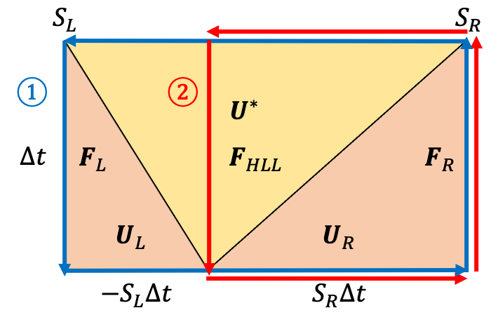
So before we get into the HLLD method, let's talk about the simpler HLL method (we'll use this result later). The solution to the Lehman problem is that various waves spread from the center, but the HLL method considers only two types of waves, the leftward wave $ S_L $ and the rightward wave $ S_R $. In addition, $ \ mathbf {U} $ approximates constant ** within the region surrounded by two waves (Lehman fan). For these two waves, select the fastest magnetic sound wave to the left and right, and the speed is

S_L = \mathrm{min}\left(u_L-{c_{fx}}_L, u_R-{c_{fx}}_R\right), S_R = \mathrm{max}\left(u_L+{c_{fx}}_L, u_R+{c_{fx}}_R\right)

S_L = \mathrm{min}\left(u_L, u_R\right)-\mathrm{max}\left({c_{fx}}_L, {c_{fx}}_R\right), S_R = \mathrm{max}\left(u_L, u_R\right)+\mathrm{max}\left({c_{fx}}_L, {c_{fx}}_R\right)

And so on. Integrating the equation in the $ x-t $ plane using Green's theorem

\iint_S\left(\frac{\partial\mathbf{U}}{\partial t}+\frac{\partial\mathbf{F}}{\partial x}\right)dxdt = \oint_c\left(-\mathbf{U}dx+\mathbf{F}dt\right) = \mathbf{0}

Therefore, regarding the integration path ① in the figure below,

-S_R\mathbf{U}_R+S_L\mathbf{U}_L+\mathbf{F}_R-\mathbf{F}_L+\left(S_R-S_L\right)\mathbf
{U}^* = \mathbf{0}

About integration path ②

-S_R\mathbf{U}_R+\mathbf{F}_R-\mathbf{F}_{HLL}+S_R\mathbf
{U}^* = \mathbf{0}

Therefore, the intermediate states $ \ mathbf {U} ^ * $ and $ \ mathbf {F} _ {HLL} $ are

\begin{aligned}
\mathbf{U}^* &= \frac{S_R\mathbf{U}_R-S_L\mathbf{U}_L-\mathbf{F}_R+\mathbf{F}_L}{S_R-S_L} \\
\mathbf{F}_{HLL} &= \mathbf{F}_R+S_R\left(\mathbf{U}^*-\mathbf{U}_R\right) \\
&= \frac{S_R\mathbf{F}_L-S_L\mathbf{F}_R+S_R S_L\left(\mathbf{U}_R-\mathbf{U}_L\right)}{S_R-S_L}
\end{aligned}

Can be obtained.

Here, we are considering the case of $ S_L <0 <S_R $, but if $ S_L> 0 $, then $ \ mathbf {F} _L $, and if $ S_R <0 $, then $ \ mathbf. It is OK if {F} _R $ is the flux at the cell boundary.

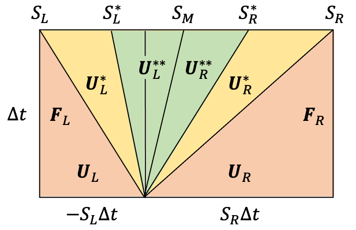
Next, let's extend the above method to derive the HLLD method. The HLLD method assumes that ** $ u $ is constant within the Lehman fan **. This also keeps $ p_T $ constant and ** excludes lagging magnetic waves **. So in this case, the solution to the Lehman problem is as shown in the figure below.

--Area faster than fast-moving magnetic sound waves x 2 --Region between fast-moving magnetic sound waves and Alfvén waves x 2 --Region between Alfvén wave and entropy wave × 2

It is divided into 6 areas.

From here, let's find $ \ mathbf {U} $ in the domain one after another. First, from the premise, the following holds.

u^*_L = u^{**}_L = u^{**}_R = u^*_R \equiv S_M

{p_T}^*_L = {p_T}^{**}_L = {p_T}^{**}_R = {p_T}^*_R \equiv {p_T}^*

$ S_M $ is calculated as follows using $ \ rho_ {HLL} $ and $ \ left (\ rho u \ right) _ {HLL} $ obtained by the HLL method.

S_M = \frac{\left(\rho u\right)_{HLL}}{\rho_{HLL}} = \frac{\left(S_R-u_R\right)\rho_R u_R-\left(S_L-u_L\right)\rho_L u_L-{p_T}_R+{p_T}_L}{\left(S_R-u_R\right)\rho_R-\left(S_L-u_L\right)\rho_L}

Jump conditions for fast-moving magnetic sound waves

First, let's see how the value changes before and after the fast-moving magnetic sound wave. For that purpose, take the integration path ① so that the area of $ \ mathbf {U} _R $ and the area of $ \ mathbf {U} ^ * _R $ are included in half as shown in the figure below.

At this time

S_R\mathbf{U}_R-\mathbf{F}\left(\mathbf{U}_R\right) = S_R\mathbf{U}^*_R-\mathbf{F}\left(\mathbf{U}^*_R\right)

So, if you write this concretely in terms of ingredients, it will be as follows.

S_R\begin{bmatrix}
\rho_R \\
\rho_R u_R \\
\rho_R v_R \\
\rho_R w_R \\
{B_y}_R \\
{B_z}_R \\
e_R
\end{bmatrix}
-
\begin{bmatrix}
\rho_R u_R \\
\rho_R u_R^2+{p_T}_R-B_x^2 \\
\rho_R u_R v_R-B_x{B_y}_R \\
\rho_R u_R w_R-B_x{B_z}_R \\
{B_y}_R u_R-B_x v_R \\
{B_z}_R u_R-B_x w_R \\
\left(e_R+{p_T}_R\right)u_R-B_x \left(\mathbf{v}_R\cdot\mathbf{B}_R\right)
\end{bmatrix}
=
S_R\begin{bmatrix}
\rho^*_R \\
\rho^*_R S_M \\
\rho^*_R v^*_R \\
\rho^*_R w^*_R \\
{B_y}^*_R \\
{B_z}^*_R \\
e^*_R
\end{bmatrix}
-
\begin{bmatrix}
\rho^*_R S_M \\
\rho^*_R S_M^2+{p_T}^*-B_x^2 \\
\rho^*_R S_M v^*_R-B_x{B_y}^*_R \\
\rho^*_R S_M w^*_R-B_x{B_z}^*_R \\
{B_y}^*_R S_M-B_x v^*_R \\
{B_z}^*_R S_M-B_x w^*_R \\
\left(e^*_R+{p_T}^*\right)S_M-B_x \left(\mathbf{v}^*_R\cdot\mathbf{B}^*_R\right)
\end{bmatrix}

By thinking about the left side in the same way, $ \ mathbf {U} ^ * _ \ alpha $ can be obtained as follows. $ \ Alpha $ means L or R.

\begin{aligned}
\rho^*_\alpha &= \rho_\alpha\frac{S_\alpha-u_\alpha}{S_\alpha-S_M} \\
v^*_\alpha &= v_\alpha-B_x {B_y}_\alpha\frac{S_M-u_\alpha}{\rho_\alpha\left(S_\alpha-u_\alpha\right)\left(S_\alpha-S_M\right)-B_x^2} \\
w^*_\alpha &= w_\alpha-B_x {B_z}_\alpha\frac{S_M-u_\alpha}{\rho_\alpha\left(S_\alpha-u_\alpha\right)\left(S_\alpha-S_M\right)-B_x^2} \\
{B_y}^*_\alpha &= {B_y}_\alpha\frac{\rho_\alpha\left(S_\alpha-u_\alpha\right)^2-B_x^2}{\rho_\alpha\left(S_\alpha-u_\alpha\right)\left(S_\alpha-S_M\right)-B_x^2} \\
{B_z}^*_\alpha &= {B_z}_\alpha\frac{\rho_\alpha\left(S-u_\alpha\right)^2-B_x^2}{\rho_\alpha\left(S_\alpha-u_\alpha\right)\left(S_\alpha-S_M\right)-B_x^2}
\end{aligned}

\begin{aligned}
p_T^* &= {p_T}_L+\rho_L\left(S_L-u_L\right)\left(S_M-u_L\right) \\
&= {p_T}_R+\rho_R\left(S_R-u_R\right)\left(S_M-u_R\right) \\
&= \frac{\left(S_R-u_R\right)\rho_R{p_T}_L-\left(S_L-u_L\right)\rho_L{p_T}_R+\rho_L\rho_R\left(S_R-u_R\right)\left(S_L-u_L\right)\left(u_R-u_L\right)}{\left(S_R-u_R\right)\rho_R-\left(S_L-u_L\right)\rho_L}
\end{aligned}

e^*_\alpha = \frac{\left(S_\alpha-u_\alpha\right)e_\alpha-{p_T}_\alpha u_\alpha+p_T^*S_M+B_x\left(\mathbf{v}_\alpha\cdot\mathbf{B}_\alpha-\mathbf{v}^*_\alpha\cdot\mathbf{B}^*_\alpha\right)}{S_\alpha-S_M}

Jump conditions for Alfvén waves

Next, in order to see the change before and after the Alfvén wave, half the integration path ② is divided into the area of $ \ mathbf {U} ^ \ * _ R $ and the area of $ \ mathbf {U} ^ {\ * \ *} Make sure that the area of _R $ is included.

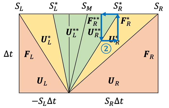
Where $ S ^ {\ *} \ _ L $ and $ S ^ {\ *} \ _R $ are

S^*_L = S_M-\frac{|B_x|}{\sqrt{\rho^*_L}},\ S^*_R = S_M+\frac{|B_x|}{\sqrt{\rho^*_R}}

I will take it. In the same way as in the case of integration path ①

S^*_R\mathbf{U}^*_R-\mathbf{F}\left(\mathbf{U}^*_R\right) = S^*_R\mathbf{U}^{**}_R-\mathbf{F}\left(\mathbf{U}^{**}_R\right)

S^*_R\begin{bmatrix}
\rho^*_R \\
\rho^*_R S_M \\
\rho^*_R v^*_R \\
\rho^*_R w^*_R \\
{B_y}^*_R \\
{B_z}^*_R \\
e^*_R
\end{bmatrix}
-
\begin{bmatrix}
\rho^*_R S_M \\
\rho^*_R S_M^2+{p_T}^*-B_x^2 \\
\rho^*_R S_M v^*_R-B_x{B_y}^*_R \\
\rho^*_R S_M w^*_R-B_x{B_z}^*_R \\
{B_y}^*_R S_M-B_x v^*_R \\
{B_z}^*_R S_M-B_x w^*_R \\
\left(e^*_R+{p_T}^*\right)S_M-B_x \left(\mathbf{v}^*_R\cdot\mathbf{B}^*_R\right)
\end{bmatrix}
=
S^*_R\begin{bmatrix}
\rho^{**}_R \\
\rho^{**}_R S_M \\
\rho^{**}_R v^{**}_R \\
\rho^{**}_R w^{**}_R \\
{B_y}^{**}_R \\
{B_z}^{**}_R \\
e^{**}_R
\end{bmatrix}
-
\begin{bmatrix}
\rho^{**}_R S_M \\
\rho^{**}_R S_M^2+{p_T}^*-B_x^2 \\
\rho^{**}_R S_M v^{**}_R-B_x{B_y}^{**}_R \\
\rho^{**}_R S_M w^{**}_R-B_x{B_z}^{**}_R \\
{B_y}^{**}_R S_M-B_x v^{**}_R \\
{B_z}^{**}_R S_M-B_x w^{**}_R \\
\left(e^{**}_R+{p_T}^*\right)S_M-B_x \left(\mathbf{v}^{**}_R\cdot\mathbf{B}^{**}_R\right)
\end{bmatrix}

It will be. From here you can only see the following $ \ rho ^ {**} _ \ alpha $.

\rho^{**}_\alpha = \rho^*_\alpha

Jump conditions for entropy waves

Furthermore, consider the integration path ③ in the figure below.

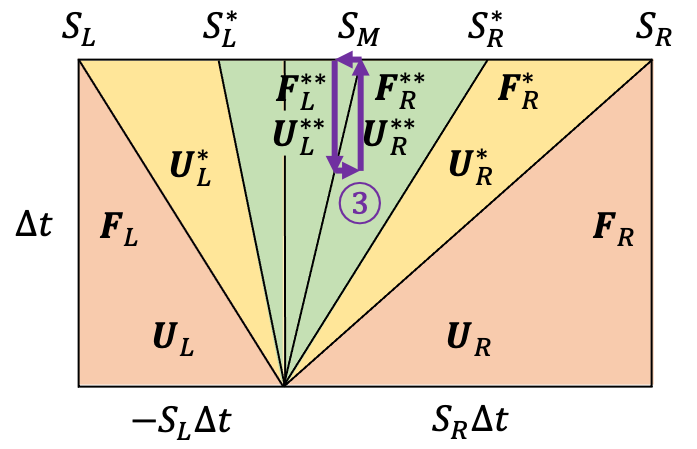
S_M\mathbf{U}^{**}_L-\mathbf{F}\left(\mathbf{U}^{**}_L\right) = S_M\mathbf{U}^{**}_R-\mathbf{F}\left(\mathbf{U}^{**}_R\right)

S_M\begin{bmatrix}
\rho^*_L \\
\rho^*_L S_M \\
\rho^*_L v^{**}_L \\
\rho^*_L w^{**}_L \\
{B_y}^{**}_L \\
{B_z}^{**}_L \\
e^{**}_L
\end{bmatrix}
-
\begin{bmatrix}
\rho^*_L S_M \\
\rho^*_L S_M^2+{p_T}^*-B_x^2 \\
\rho^*_L S_M v^{**}_L-B_x{B_y}^{**}_L \\
\rho^*_L S_M w^{**}_L-B_x{B_z}^{**}_L \\
{B_y}^{**}_L S_M-B_x v^{**}_L \\
{B_z}^{**}_L S_M-B_x w^{**}_L \\
\left(e^{**}_L+{p_T}^*\right)S_M-B_x \left(\mathbf{v}^{**}_L\cdot\mathbf{B}^{**}_L\right)
\end{bmatrix}

=
S_M\begin{bmatrix}
\rho^*_R \\
\rho^*_R S_M \\
\rho^*_R v^{**}_R \\
\rho^*_R w^{**}_R \\
{B_y}^{**}_R \\
{B_z}^{**}_R \\
e^{**}_R
\end{bmatrix}
-
\begin{bmatrix}
\rho^*_R S_M \\
\rho^*_R S_M^2+{p_T}^*-B_x^2 \\
\rho^*_R S_M v^{**}_R-B_x{B_y}^{**}_R \\
\rho^*_R S_M w^{**}_R-B_x{B_z}^{**}_R \\
{B_y}^{**}_R S_M-B_x v^{**}_R \\
{B_z}^{**}_R S_M-B_x w^{**}_R \\
\left(e^{**}_R+{p_T}^*\right)S_M-B_x \left(\mathbf{v}^{**}_R\cdot\mathbf{B}^{**}_R\right)
\end{bmatrix}

From here, $ v ^ {\ * \ *} $, $ w ^ {\ * \ *} $, $ {B_y} ^ {\ * \ *} $, $ {B_z} ^ {\ * \ *} Indicates that $ is equal on the left and right.

\begin{aligned}
v^{**}_L &= v^{**}_R \equiv v^{**} \\
w^{**}_L &= w^{**}_R \equiv w^{**} \\
{B_y}^{**}_L &= {B_y}^{**}_R \equiv {B_y}^{**} \\
{B_z}^{**}_L &= {B_z}^{**}_R \equiv {B_z}^{**}
\end{aligned}

Based on this, this time, integrate with the integration path ④ in the figure below.

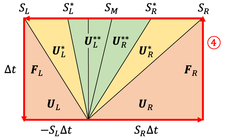
\begin{aligned}
\mathbf{0} &= -S_R\mathbf{U}_R+S_L\mathbf{U}_L+\mathbf{F}_R-\mathbf{F}_L+\left(S_R-S^*_R\right)\mathbf{U}^*_R+\left(S^*_L-S_L\right)\mathbf{U}^*_L+\left(S^*_R-S_M\right)\mathbf{U}^{**}_R+\left(S_M-S^*_L\right)\mathbf{U}^{**}_L \\
&= -S^*_R\mathbf{U}^*_R+S^*_L\mathbf{U}^*_L+\mathbf{F}^*_R-\mathbf{F}^*_L+\left(S^*_R-S_M\right)\mathbf{U}^{**}_R+\left(S_M-S^*_L\right)\mathbf{U}^{**}_L \\
&= -\left(S_M+\frac{|B_x|}{\sqrt{\rho^*_R}}\right)\mathbf{U}^*_R+\left(S_M-\frac{|B_x|}{\sqrt{\rho^*_L}}\right)\mathbf{U}^*_L+\mathbf{F}^*_R-\mathbf{F}^*_L+\frac{|B_x|}{\sqrt{\rho^*_R}}\mathbf{U}^{**}_R+\frac{|B_x|}{\sqrt{\rho^*_L}}\mathbf{U}^{**}_L
\end{aligned}

from here,

\begin{aligned}
v^{**} &= \frac{\sqrt{\rho^*_L}v^*_L+\sqrt{\rho^*_R}v^*_R+\left({B_y}^*_R-{B_y}^*_L\right)\mathrm{sign}\left(B_x\right)}{\sqrt{\rho^*_L}+\sqrt{\rho^*_R}} \\
w^{**} &= \frac{\sqrt{\rho^*_L}w^*_L+\sqrt{\rho^*_R}w^*_R+\left({B_z}^*_R-{B_z}^*_L\right)\mathrm{sign}\left(B_x\right)}{\sqrt{\rho^*_L}+\sqrt{\rho^*_R}} \\
B_y^{**} &= \frac{\sqrt{\rho^*_L}{B_y}^*_R+\sqrt{\rho^*_R}{B_y}^*_L+\sqrt{\rho^*_L\rho^*_R}\left(v^*_R-v^*_L\right)\mathrm{sign}\left(B_x\right)}{\sqrt{\rho^*_L}+\sqrt{\rho^*_R}} \\
B_z^{**} &= \frac{\sqrt{\rho^*_L}{B_z}^*_R+\sqrt{\rho^*_R}{B_z}^*_L+\sqrt{\rho^*_L\rho^*_R}\left(w^*_R-w^*_L\right)\mathrm{sign}\left(B_x\right)}{\sqrt{\rho^*_L}+\sqrt{\rho^*_R}}
\end{aligned}

Finally, by using the jump condition for the Alfvén wave again, we get:

e^{**}_\alpha = e^*_\alpha\mp\sqrt{\rho^*_\alpha}\left(\mathbf{v}^*_\alpha\cdot\mathbf{B}^*_\alpha-\mathbf{v}^{**}\cdot\mathbf{B}^{**}\right)\mathrm{sign}\left(B_x\right)

The compound number takes a minus when it is L and a plus when it is R.

It's been long, but now we have all the $ \ mathbf {U} $ in each area. The following formula is finally obtained by summarizing the above.

\mathbf{F}_{HLLD} = \begin{cases}
\mathbf{F}_L & (0 < S_L) \\
\mathbf{F}_L^* & (S_L \le 0 < S_L^*) \\
\mathbf{F}_L^{**} & (S_L^* \le 0 < S_M) \\
\mathbf{F}_R^{**} & (S_M \le 0 < S_R^*) \\
\mathbf{F}_R^* & (S_R^* \le 0 < S_R) \\
\mathbf{F}_R & (S_R < 0)
\end{cases}

Multidimensional

In order to make it multidimensional, it seems that the HLLD method should be applied to each of the $ x, y, z $ directions, but in reality it is not so simple, but the difficulty of magnetic fluid calculation It is one of. The problem here is the divergence of the magnetic field. Originally, from Maxwell's equations, the magnetic field is always non-divergent, that is,

\nabla\cdot\mathbf{B} = 0

It must be, but in the case of numerical calculations, errors can break this, and sometimes it has the negative effect of breaking the calculation. There are two ways to avoid this.

--A method that does not generate magnetic field divergence from the beginning by devising the arrangement etc. --How to suppress the magnetic field divergence generated by modifying the equation

There are two types. The former is famous for the CT method. In the latter, the projection method and the 9 wave method are known, and here we will introduce the 9 wave method, which is relatively simple to implement.

9 wave method

Using the method proposed by Dedner et al. (2002), we introduce a new variable called $ \ psi $ and extend the equation as follows:

\frac{\partial\mathbf{U}}{\partial t} + \frac{\partial\mathbf{F}}{\partial x} + \frac{\partial\mathbf{G}}{\partial y} + \frac{\partial\mathbf{H}}{\partial z} = \mathbf{S}

\mathbf{U} = \begin{bmatrix}
\rho \\
\rho u \\
\rho v \\
\rho w \\
B_x \\
B_y \\
B_z \\
e \\
\psi
\end{bmatrix},\ 
\mathbf{F} = \begin{bmatrix}
\rho u \\
\rho u^2+p_T-B_x^2 \\
\rho uv-B_xB_y \\
\rho uw-B_xB_z \\
\psi \\
B_yu-B_xv \\
B_zu-B_xw \\
\left(e+p_T\right)u-B_x\left(\mathbf{v}\cdot\mathbf{B}\right) \\
c_h^2 B_x
\end{bmatrix},\ 
\mathbf{G} = \begin{bmatrix}
\rho v \\
\rho vu-B_yB_x \\
\rho v^2+p_T-B_y^2 \\
\rho vw-B_yB_z \\
B_xv-B_yu \\
\psi \\
B_zv-B_yw \\
\left(e+p_T\right)v-B_y\left(\mathbf{v}\cdot\mathbf{B}\right) \\
c_h^2 B_y
\end{bmatrix},\ 
\mathbf{H} = \begin{bmatrix}
\rho w \\
\rho wu-B_zB_x \\
\rho wv-B_zB_y \\
\rho w^2+p_T-B_z^2 \\
B_xw-B_zu \\
B_yw-B_zv \\
\psi \\
\left(e+p_T\right)w-B_z\left(\mathbf{v}\cdot\mathbf{B}\right) \\
c_h^2 B_z
\end{bmatrix},\ 
\mathbf{S} = \begin{bmatrix}
0 \\
0 \\
0 \\
0 \\
0 \\
0 \\
0 \\
0 \\
-\frac{c_h^2}{c_p^2}\psi
\end{bmatrix}

This $ \ psi $ is an artificially introduced variable to suppress magnetic field divergence, so it has no physical meaning.

Find $ B_x $ and $ \ psi $ at the cell boundaries as follows:

\begin{aligned}
{B_x}_M &= {B_x}_L+\frac{1}{2}\left({B_x}_R-{B_x}_L\right)-\frac{1}{2c_h}\left(\psi_R-\psi_L\right) \\
\psi_M &= \psi_L+\frac{1}{2}\left(\psi_R-\psi_L\right)-\frac{c_h}{2}\left({B_x}_R-{B_x}_L\right)
\end{aligned}

In the actual calculation, instead of calculating the source term of $ \ psi $ as it is, once forget the source term and find $ \ psi ^ * $ from the difference in flux like other variables, then do as follows. It is common to find $ \ psi ^ {n + 1} $.

\psi^{n+1} = \psi^*\exp\left(-\Delta t_n\frac{c_h^2}{c_p^2}\right)

Note that $ c_h $ and $ c_p $ that appear here are free parameters that represent the speed of artificial propagation and attenuation for $ \ nabla \ cdot \ mathbf {B} $ and $ \ psi $. The maximum speed allowed by the CFL condition as $ c_h $,

c_h = \mathrm{CFL}\cdot\mathrm{min}\left(\Delta x, \Delta y, \Delta z\right)/\Delta t_n

It seems that it is best to select $ c_r = 0.18 $ after making $ c_r = c_p ^ 2/c_h $ a constant for $ c_p $, regardless of the spatial resolution.

High accuracy

When finding $ \ mathbf {F} \ _ {i + 1/2} $, use $ \ mathbf {U} \ _i $ as $ \ mathbf {U} \ _L $ and $ \ mathbf {U} \ _R $ Choosing $ \ mathbf {U} \ _ {i + 1} $ as is equivalent to the so-called ** leeward difference **, which is the first-order spatial accuracy. As I will show you later, this is actually a solution with large numerical diffusion and quite blurry. Therefore, here we will introduce a method to improve spatial accuracy. Also, regarding the time accuracy, the same can be considered for the partial differential equation, just as the accuracy was improved by using the Runge-Kutta method for the ordinary differential equation.

~~ (It's getting longer and tired ...) ~~

Higher precision of space

For example as $ {\ mathbf {U} _ {i + 1/2}} _L $

{\mathbf{U}_{i+1/2}}_L = \frac{-\mathbf{U}_{i-1}+4\mathbf{U}_i+\mathbf{U}_{i+1}}{4}

Spatial quadratic precision can be obtained by using, but it is not very preferable to simply combine $ \ mathbf {U} $ linearly in this way because numerical vibration will occur. Therefore, various nonlinear schemes have been devised to avoid this. Here, we will briefly introduce MUSCL with 2nd precision and MP5 with 5th precision.

MUSCL With the method proposed by van Leer (1979), by introducing a limiter as shown below, it is possible to reduce the accuracy to the primary accuracy so that numerical vibration does not occur on the discontinuous surface while basically maintaining the secondary accuracy. I will.

\begin{aligned}
{\mathbf{U}_{i+1/2}}_L &= \mathbf{U}_i+\frac{1}{2}\Delta_i \\
{\mathbf{U}_{i-1/2}}_R &= \mathbf{U}_i-\frac{1}{2}\Delta_i
\end{aligned}

\Delta_i = \mathrm{limiter}\left(\mathbf{U}_{i+1}-\mathbf{U}_i, \mathbf{U}_i-\mathbf{U}_{i-1}\right)

It seems that the following minmod (Roe, 1986) and MC (van Leer, 1977) are often used as limiters.

\begin{aligned}
\mathrm{minmod}\left(a, b\right) &= \frac{1}{2}\left[\mathrm{sign}\left(a\right)+\mathrm{sign}\left(b\right)\right]\mathrm{min}\left(|a|, |b|\right) \\
\mathrm{MC}\left(a, b\right) &= \frac{1}{2}\left[\mathrm{sign}\left(a\right)+\mathrm{sign}\left(b\right)\right]\mathrm{min}\left(2|a|, \frac{|a+b|}{2}, 2|b|\right)
\end{aligned}

MP5 This is the method by Suresh and Huynh (1997). First, interpolate $ {\ mathbf {U} _ {i + 1/2}} _L $ with a linear scheme with 5th order precision.

{\mathbf{U}_{i+1/2}}^*_L = \frac{2\mathbf{U}_{i-2}-13\mathbf{U}_{i-1}+47\mathbf{U}_i+27\mathbf{U}_{i+1}-3\mathbf{U}_{i+2}}{60}

Of course, numerical vibration will occur if nothing is done, so a certain lower limit $ \ mathbf {U} \ _ {\ mathrm {min}} $ and an upper limit $ \ mathbf {U} \ _ {\ mathrm {max}} $ And use their median to find $ {\ mathbf {U} \ _ {i + 1/2}} _L $.

{\mathbf{U}_{i+1/2}}_L = \mathrm{median}\left({\mathbf{U}_{i+1/2}}^*_L, \mathbf{U}_{\mathrm{min}}, \mathbf{U}_{\mathrm{max}}\right)

The specific methods for finding $ \ mathbf {U} \ _ {\ mathrm {min}} $ and $ \ mathbf {U} \ _ {\ mathrm {max}} $ are quite long, so they are omitted here.

Higher time accuracy

\frac{d\mathbf{U}}{dt} = L\left(\mathbf{U}\right)

When it can be written, the solution as follows is equivalent to the so-called ** Euler method **, which is the first-order time accuracy.

\mathbf{U}^{n+1} = \mathbf{U}^n+\Delta tL\left(\mathbf{U}^n\right)

However, this can also be improved by using the Runge-Kutta method. This time, I will post the ** SSPRK (strong stability preserving Runge-Kutta) ** series (Shu and Osher, 1988), which has good properties in the sense that it does not generate extra numerical vibrations among the Runge-Kutta methods. ..

Secondary accuracy SSPRK (2, 2)

\begin{aligned}
\mathbf{U}^{\left(1\right)} &= \mathbf{U}^n+\Delta tL\left(\mathbf{U}^n\right) \\
\mathbf{U}^{n+1} &= \frac{1}{2}\mathbf{U}^n+\frac{1}{2}\mathbf{U}^{\left(1\right)}+\frac{1}{2}\Delta tL\left(\mathbf{U}^{\left(1\right)}\right)
\end{aligned}

Third-order accuracy SSPRK (3, 3)

\begin{aligned}
\mathbf{U}^{\left(1\right)} &= \mathbf{U}^n+\Delta tL\left(\mathbf{U}^n\right) \\
\mathbf{U}^{\left(2\right)} &= \frac{3}{4}\mathbf{U}^n+\frac{1}{4}\mathbf{U}^{\left(1\right)}+\frac{1}{4}\Delta tL\left(\mathbf{U}^{\left(1\right)}\right) \\
\mathbf{U}^{n+1} &= \frac{1}{3}\mathbf{U}^n+\frac{2}{3}\mathbf{U}^{\left(2\right)}+\frac{2}{3}\Delta tL\left(\mathbf{U}^{\left(2\right)}\right)
\end{aligned}

result

Based on the above, the results calculated using MP5 and SSPRK (3, 3) are as follows. The following are all calculated with the number of divisions $ N_x \ times N_y = 200 \ times 200 $, $ \ mathrm {CFL} = 0.4 $.

Above is a pressure plot. You can see all the variables by opening the fold.

Video

--Pressure

density
u
v
B_x
B_y
\psi

image

--Pressure

density
u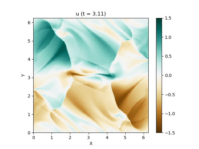
v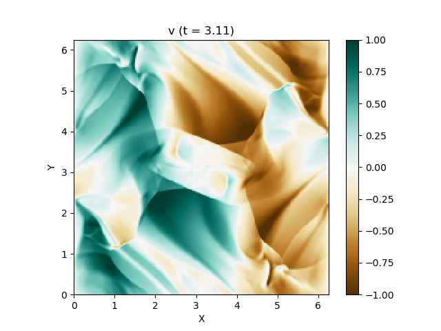
B_x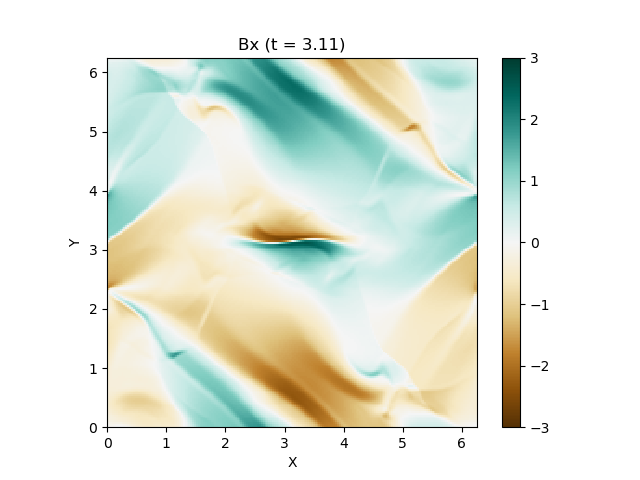
B_y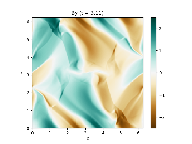
\psi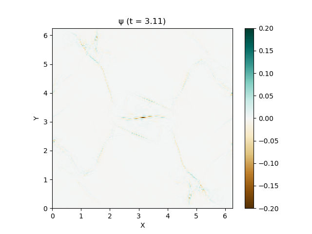

Good feeling!

Differences by scheme

Let's take a look at the differences depending on the scheme. Let's compare the following three types.

--Upwind difference / Euler method (spatial first-order, time first-order) --MUSCL-minmod ・ SSPRK (2, 2) (Spatial secondary / Time secondary) --MP5 / SSPRK (3, 3) (Spatial 5th / Time 3rd)

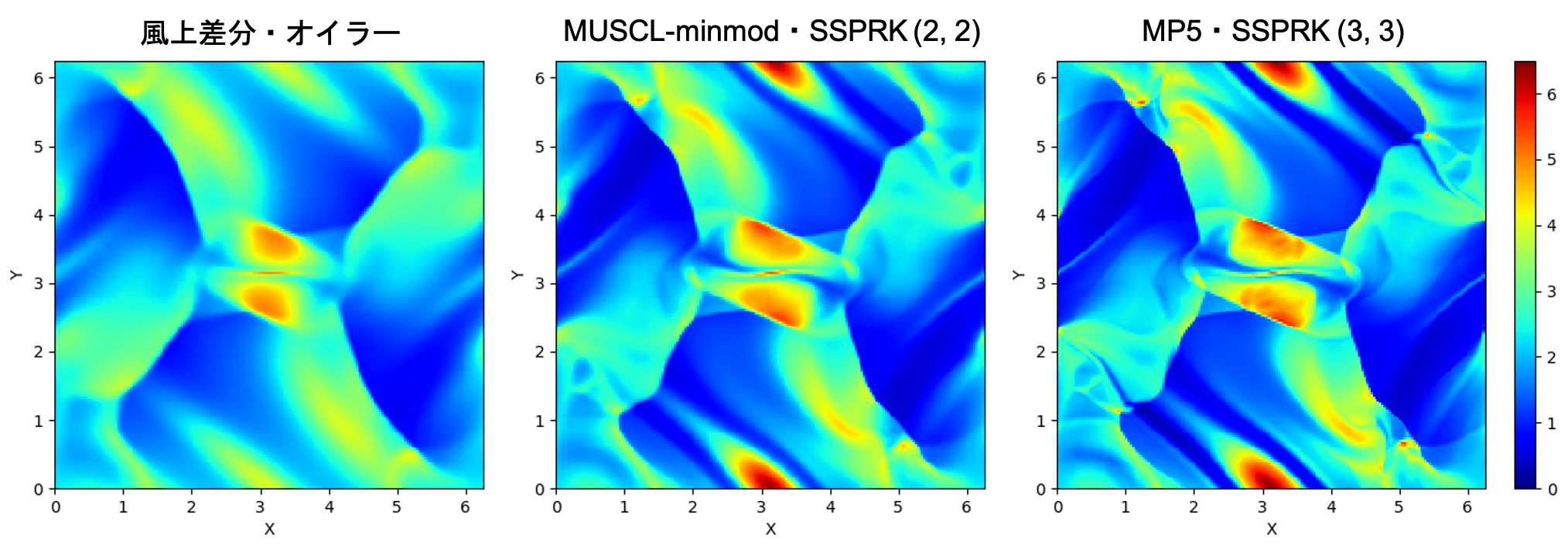
There is a clear difference when you try this. In particular, the windward difference / Euler method should have the same spatial resolution, but it is quite blurred.

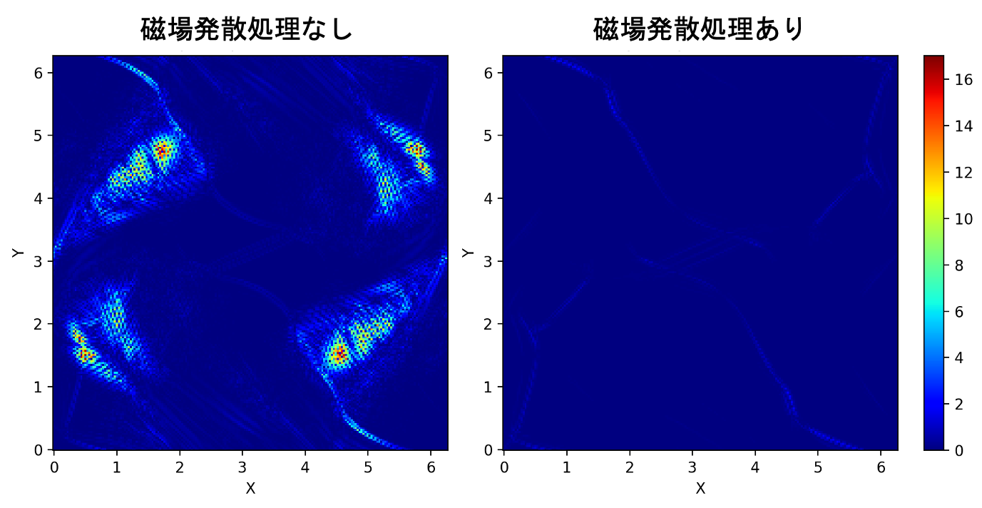
Difference with and without magnetic field divergence treatment

Next, let's see what happens if the magnetic field divergence process is not added. We will compare the difference between the two with MUSCL-minmod / SSPRK (2, 2), which was the easiest to see.

...

It broke down without the magnetic field divergence treatment. .. ..

For the time being, let's compare the figures just before the calculation breaks.

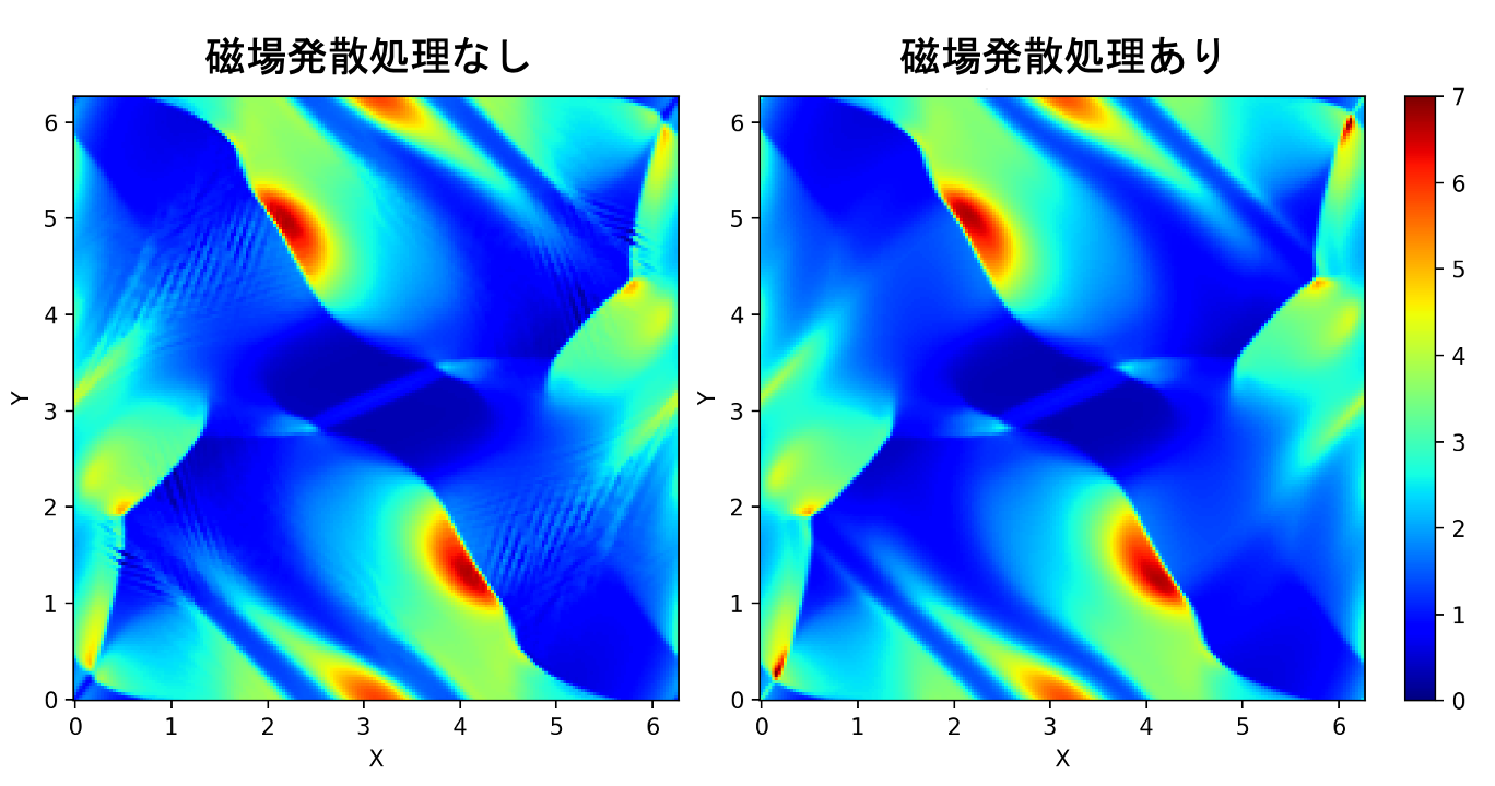
On the left, you can see a suspicious striped pattern that seems to be dangerous. \|\nabla\cdot\mathbf{B}\|If you plot, you can see that a large magnetic field divergence has occurred just there. On the other hand, it is well suppressed on the right.

Source code

At the moment, we are creating two versions of C ++ and Python, which are available on GutHub. The C ++ version uses OpenMP parallelization, which makes it suitable for large size calculations such as $ N_x \ times N_y = 200 \ times 200 $. Since constexpr if statement and Structured binding are used, C ++ 17 or higher is required for compilation. On the other hand, in the Python version, I made it to plot immediately on the spot, so if you want to see the result quickly, I think this is good. Even though Python is said, the for statement is eliminated and NumPy is left to calculate as much as possible, so it should be a decent performance. .. .. Since it will be long, only the Python version is listed here.

Python version source code

`main.py`


import time
import numpy as np
import matplotlib.pyplot as plt
import matplotlib.cm as cm

#Number of grids
#XN = 200; YN = 200
XN = 100; YN = 100
#Number of file outputs
PN = 100
#Number of storage variables
VN = 9
#Computation area size
XL = 2.0*np.pi; YL = 2.0*np.pi
TL = np.pi
#Grid size
dx = XL/XN; dy = YL/YN
#CFL number
CFL = 0.4
#Specific heat ratio
gam = 5.0/3.0
#Parameters for suppressing magnetic field divergence(Dedner et al., 2002)
cr = 0.18

#MINMOD function
def minmod(a, b):
    return 0.5*(np.sign(a)+np.sign(b))*np.minimum(np.abs(a), np.abs(b))
#Median
def median(a, b, c):
    return a+minmod(b-a, c-a)
#x-direction flux
def mhdfx(rho, u, v, w, bx, by, bz, e, psi, pt, ch):
    fx = np.zeros((XN, YN, VN))
    fx[:, :, 0] = rho*u
    fx[:, :, 1] = rho*u*u+pt-bx*bx
    fx[:, :, 2] = rho*v*u-bx*by
    fx[:, :, 3] = rho*w*u-bx*bz
    fx[:, :, 4] = psi
    fx[:, :, 5] = by*u-bx*v
    fx[:, :, 6] = bz*u-bx*w
    fx[:, :, 7] = (e+pt)*u-bx*(u*bx+v*by+w*bz)
    fx[:, :, 8] = ch*ch*bx
    return fx
#y-direction flux
def mhdfy(rho, u, v, w, bx, by, bz, e, psi, pt, ch):
    fy = np.zeros((XN, YN, VN))
    fy[:, :, 0] = rho*v
    fy[:, :, 1] = rho*u*v-by*bx
    fy[:, :, 2] = rho*v*v+pt-by*by
    fy[:, :, 3] = rho*w*v-by*bz
    fy[:, :, 4] = bx*v-by*u
    fy[:, :, 5] = psi
    fy[:, :, 6] = bz*v-by*w
    fy[:, :, 7] = (e+pt)*v-by*(u*bx+v*by+w*bz)
    fy[:, :, 8] = ch*ch*by
    return fy
#HLLD Lehman solver(Miyoshi and Kusano, 2005)
def hlldx(ql, qr, ch):
    #density
    rhol = ql[:, :, 0]
    rhor = qr[:, :, 0]
    #Momentum
    mxl = ql[:, :, 1]
    myl = ql[:, :, 2]
    mzl = ql[:, :, 3]
    mxr = qr[:, :, 1]
    myr = qr[:, :, 2]
    mzr = qr[:, :, 3]
    #magnetic field
    bxl = ql[:, :, 4]
    byl = ql[:, :, 5]
    bzl = ql[:, :, 6]
    bxr = qr[:, :, 4]
    byr = qr[:, :, 5]
    bzr = qr[:, :, 6]
    #energy
    el = ql[:, :, 7]
    er = qr[:, :, 7]
    #Artificial potential for suppressing magnetic field divergence(Dedner et al., 2002)
    psil = ql[:, :, 8]
    psir = qr[:, :, 8]
    #speed
    ul = mxl/rhol
    vl = myl/rhol
    wl = mzl/rhol
    ur = mxr/rhor
    vr = myr/rhor
    wr = mzr/rhor
    # (Thermal)pressure
    pl = (gam-1.0)*(el-0.5*rhol*(ul*ul+vl*vl+wl*wl)-0.5*(bxl*bxl+byl*byl+bzl*bzl))
    pr = (gam-1.0)*(er-0.5*rhor*(ur*ur+vr*vr+wr*wr)-0.5*(bxr*bxr+byr*byr+bzr*bzr))
    ptl = pl+0.5*(bxl*bxl+byl*byl+bzl*bzl)
    #Total pressure(Thermal pressure+Magnetic pressure)
    ptr = pr+0.5*(bxr*bxr+byr*byr+bzr*bzr)
    #Speed of sound
    al = np.sqrt(gam*pl/rhol)
    ar = np.sqrt(gam*pr/rhor)
    #Alfvén speed
    cal = np.sqrt((bxl*bxl+byl*byl+bzl*bzl)/rhol)
    car = np.sqrt((bxr*bxr+byr*byr+bzr*bzr)/rhor)
    caxl = np.sqrt(bxl*bxl/rhol)
    caxr = np.sqrt(bxr*bxr/rhor)
    #Fast-moving magnetic sound wave speed
    cfl = np.sqrt(0.5*(al*al+cal*cal+np.sqrt((al*al+cal*cal)**2-4.0*(al*caxl)**2)))
    cfr = np.sqrt(0.5*(ar*ar+car*car+np.sqrt((ar*ar+car*car)**2-4.0*(ar*caxr)**2)))
    sfl = np.minimum(ul-cfl, ur-cfr)
    sfr = np.maximum(ul+cfl, ur+cfr)
    sm = ((sfr-ur)*rhor*ur-(sfl-ul)*rhol*ul-ptr+ptl)/((sfr-ur)*rhor-(sfl-ul)*rhol)
    um = sm
    bxm = bxl+0.5*(bxr-bxl)-0.5/ch*(psir-psil)
    psim = psil+0.5*(psir-psil)-0.5*ch*(bxr-bxl)
    #Lehman fan outside
    ptm = ((sfr-ur)*rhor*ptl-(sfl-ul)*rhol*ptr+rhol*rhor*(sfr-ur)*(sfl-ul)*(ur-ul))/((sfr-ur)*rhor-(sfl-ul)*rhol)
    rhoml = rhol*(sfl-ul)/(sfl-sm)
    rhomr = rhor*(sfr-ur)/(sfr-sm)
    vol = vl-bxm*byl*(sm-ul)/(rhol*(sfl-ul)*(sfl-sm)-bxm*bxm)
    vor = vr-bxm*byr*(sm-ur)/(rhor*(sfr-ur)*(sfr-sm)-bxm*bxm)
    wol = wl-bxm*bzl*(sm-ul)/(rhol*(sfl-ul)*(sfl-sm)-bxm*bxm)
    wor = wr-bxm*bzr*(sm-ur)/(rhor*(sfr-ur)*(sfr-sm)-bxm*bxm)
    byol = byl*(rhol*(sfl-ul)*(sfl-ul)-bxm*bxm)/(rhol*(sfl-ul)*(sfl-sm)-bxm*bxm)
    byor = byr*(rhor*(sfr-ur)*(sfr-ur)-bxm*bxm)/(rhor*(sfr-ur)*(sfr-sm)-bxm*bxm)
    bzol = bzl*(rhol*(sfl-ul)*(sfl-ul)-bxm*bxm)/(rhol*(sfl-ul)*(sfl-sm)-bxm*bxm)
    bzor = bzr*(rhor*(sfr-ur)*(sfr-ur)-bxm*bxm)/(rhor*(sfr-ur)*(sfr-sm)-bxm*bxm)
    eol = ((sfl-ul)*el-ptl*ul+ptm*sm+bxm*(ul*bxl+vl*byl+wl*bzl-um*bxm-vol*byol-wol*bzol))/(sfl-sm)
    eor = ((sfr-ur)*er-ptr*ur+ptm*sm+bxm*(ur*bxr+vr*byr+wr*bzr-um*bxm-vor*byor-wor*bzor))/(sfr-sm)
    srrhoml = np.sqrt(rhoml)
    srrhomr = np.sqrt(rhomr)
    sal = sm-np.sqrt(bxm*bxm/rhoml)
    sar = sm+np.sqrt(bxm*bxm/rhomr)
    #Inside the Lehman fan
    vi = (srrhoml*vol+srrhomr*vor+(byor-byol)*np.sign(bxm))/(srrhoml+srrhomr)
    wi = (srrhoml*wol+srrhomr*wor+(bzor-bzol)*np.sign(bxm))/(srrhoml+srrhomr)
    byi = (srrhoml*byor+srrhomr*byol+srrhoml*srrhomr*(vor-vol)*np.sign(bxm))/(srrhoml+srrhomr)
    bzi = (srrhoml*bzor+srrhomr*bzol+srrhoml*srrhomr*(wor-wol)*np.sign(bxm))/(srrhoml+srrhomr)
    eil = eol-srrhoml*(vol*byol+wol*bzol-vi*byi-wi*bzi)*np.sign(bxm)
    eir = eor+srrhomr*(vor*byor+wor*bzor-vi*byi-wi*bzi)*np.sign(bxm)
    fxl = mhdfx(rhol, ul, vl, wl, bxm, byl, bzl, el, psim, ptl, ch)
    fxol = mhdfx(rhoml, um, vol, wol, bxm, byol, bzol, eol, psim, ptm, ch)
    fxil = mhdfx(rhoml, um, vi, wi, bxm, byi, bzi, eil, psim, ptm, ch)
    fxir = mhdfx(rhomr, um, vi, wi, bxm, byi, bzi, eir, psim, ptm, ch)
    fxor = mhdfx(rhomr, um, vor, wor, bxm, byor, bzor, eor, psim, ptm, ch)
    fxr = mhdfx(rhor, ur, vr, wr, bxm, byr, bzr, er, psim, ptr, ch)
    fx = np.zeros((XN, YN, VN))
    slindex = sfl > 0.0
    solindex = (0.0 >= sfl) & (sal > 0.0)
    silindex = (0.0 >= sal) & (sm > 0.0)
    sirindex = (0.0 >= sm) & (sar > 0.0)
    sorindex = (0.0 >= sar) & (sfr > 0.0)
    srindex = 0.0 >= sfr
    fx[slindex, :] = fxl[slindex, :]
    fx[solindex, :] = fxol[solindex, :]
    fx[silindex, :] = fxil[silindex, :]
    fx[sirindex, :] = fxir[sirindex, :]
    fx[sorindex, :] = fxor[sorindex, :]
    fx[srindex, :] = fxr[srindex, :]
    return fx
def hlldy(ql, qr, ch):
    #density
    rhol = ql[:, :, 0]
    rhor = qr[:, :, 0]
    #Momentum
    mxl = ql[:, :, 1]
    myl = ql[:, :, 2]
    mzl = ql[:, :, 3]
    mxr = qr[:, :, 1]
    myr = qr[:, :, 2]
    mzr = qr[:, :, 3]
    #magnetic field
    bxl = ql[:, :, 4]
    byl = ql[:, :, 5]
    bzl = ql[:, :, 6]
    bxr = qr[:, :, 4]
    byr = qr[:, :, 5]
    bzr = qr[:, :, 6]
    #energy
    el = ql[:, :, 7]
    er = qr[:, :, 7]
    #Artificial potential for suppressing magnetic field divergence(Dedner et al., 2002)
    psil = ql[:, :, 8]
    psir = qr[:, :, 8]
    #speed
    ul = mxl/rhol
    vl = myl/rhol
    wl = mzl/rhol
    ur = mxr/rhor
    vr = myr/rhor
    wr = mzr/rhor
    # (Thermal)pressure
    pl = (gam-1.0)*(el-0.5*rhol*(ul*ul+vl*vl+wl*wl)-0.5*(bxl*bxl+byl*byl+bzl*bzl))
    pr = (gam-1.0)*(er-0.5*rhor*(ur*ur+vr*vr+wr*wr)-0.5*(bxr*bxr+byr*byr+bzr*bzr))
    #Total pressure(Thermal pressure+Magnetic pressure)
    ptl = pl+0.5*(bxl*bxl+byl*byl+bzl*bzl)
    ptr = pr+0.5*(bxr*bxr+byr*byr+bzr*bzr)
    #Speed of sound
    al = np.sqrt(gam*pl/rhol)
    ar = np.sqrt(gam*pr/rhor)
    #Alfvén speed
    cal = np.sqrt((bxl*bxl+byl*byl+bzl*bzl)/rhol)
    car = np.sqrt((bxr*bxr+byr*byr+bzr*bzr)/rhor)
    cayl = np.sqrt(byl*byl/rhol)
    cayr = np.sqrt(byr*byr/rhor)
    #Fast-moving magnetic sound wave speed
    cfl = np.sqrt(0.5*(al*al+cal*cal+np.sqrt((al*al+cal*cal)**2-4.0*(al*cayl)**2)))
    cfr = np.sqrt(0.5*(ar*ar+car*car+np.sqrt((ar*ar+car*car)**2-4.0*(ar*cayr)**2)))
    sfl = np.minimum(vl-cfl, vr-cfr)
    sfr = np.maximum(vl+cfl, vr+cfr)
    sm = ((sfr-vr)*rhor*vr-(sfl-vl)*rhol*vl-ptr+ptl)/((sfr-vr)*rhor-(sfl-vl)*rhol)
    vm = sm
    bym = byl+0.5*(byr-byl)-0.5/ch*(psir-psil)
    psim = psil+0.5*(psir-psil)-0.5*ch*(byr-byl)
    #Lehman fan outside
    ptm = ((sfr-vr)*rhor*ptl-(sfl-vl)*rhol*ptr+rhol*rhor*(sfr-vr)*(sfl-vl)*(vr-vl))/((sfr-vr)*rhor-(sfl-vl)*rhol)
    rhoml = rhol*(sfl-vl)/(sfl-sm)
    rhomr = rhor*(sfr-vr)/(sfr-sm)
    wol = wl-bym*bzl*(sm-vl)/(rhol*(sfl-vl)*(sfl-sm)-bym*bym)
    wor = wr-bym*bzr*(sm-vr)/(rhor*(sfr-vr)*(sfr-sm)-bym*bym)
    uol = ul-bym*bxl*(sm-vl)/(rhol*(sfl-vl)*(sfl-sm)-bym*bym)
    uor = ur-bym*bxr*(sm-vr)/(rhor*(sfr-vr)*(sfr-sm)-bym*bym)
    bzol = bzl*(rhol*(sfl-vl)*(sfl-vl)-bym*bym)/(rhol*(sfl-vl)*(sfl-sm)-bym*bym)
    bzor = bzr*(rhor*(sfr-vr)*(sfr-vr)-bym*bym)/(rhor*(sfr-vr)*(sfr-sm)-bym*bym)
    bxol = bxl*(rhol*(sfl-vl)*(sfl-vl)-bym*bym)/(rhol*(sfl-vl)*(sfl-sm)-bym*bym)
    bxor = bxr*(rhor*(sfr-vr)*(sfr-vr)-bym*bym)/(rhor*(sfr-vr)*(sfr-sm)-bym*bym)
    eol = ((sfl-vl)*el-ptl*vl+ptm*sm+bym*(ul*bxl+vl*byl+wl*bzl-uol*bxol-vm*bym-wol*bzol))/(sfl-sm)
    eor = ((sfr-vr)*er-ptr*vr+ptm*sm+bym*(ur*bxr+vr*byr+wr*bzr-uor*bxor-vm*bym-wor*bzor))/(sfr-sm)
    srrhoml = np.sqrt(rhoml)
    srrhomr = np.sqrt(rhomr)
    sal = sm-np.sqrt(bym*bym/rhoml)
    sar = sm+np.sqrt(bym*bym/rhomr)
    #Inside the Lehman fan
    wi = (srrhoml*wol+srrhomr*wor+(bzor-bzol)*np.sign(bym))/(srrhoml+srrhomr)
    ui = (srrhoml*uol+srrhomr*uor+(bxor-bxol)*np.sign(bym))/(srrhoml+srrhomr)
    bzi = (srrhoml*bzor+srrhomr*bzol+srrhoml*srrhomr*(wor-wol)*np.sign(bym))/(srrhoml+srrhomr)
    bxi = (srrhoml*bxor+srrhomr*bxol+srrhoml*srrhomr*(uor-uol)*np.sign(bym))/(srrhoml+srrhomr)
    eil = eol-srrhoml*(uol*bxol+wol*bzol-ui*bxi-wi*bzi)*np.sign(bym)
    eir = eor+srrhomr*(uor*bxor+wor*bzor-ui*bxi-wi*bzi)*np.sign(bym)
    fyl = mhdfy(rhol, ul, vl, wl, bxl, bym, bzl, el, psim, ptl, ch)
    fyol = mhdfy(rhoml, uol, vm, wol, bxol, bym, bzol, eol, psim, ptm, ch)
    fyil = mhdfy(rhoml, ui, vm, wi, bxi, bym, bzi, eil, psim, ptm, ch)
    fyir = mhdfy(rhomr, ui, vm, wi, bxi, bym, bzi, eir, psim, ptm, ch)
    fyor = mhdfy(rhomr, uor, vm, wor, bxor, bym, bzor, eor, psim, ptm, ch)
    fyr = mhdfy(rhor, ur, vr, wr, bxr, bym, bzr, er, psim, ptr, ch)
    fy = np.zeros((XN, YN, VN))
    slindex = sfl > 0.0
    solindex = (0.0 >= sfl) & (sal > 0.0)
    silindex = (0.0 >= sal) & (sm > 0.0)
    sirindex = (0.0 >= sm) & (sar > 0.0)
    sorindex = (0.0 >= sar) & (sfr > 0.0)
    srindex = 0.0 >= sfr
    fy[slindex, :] = fyl[slindex, :]
    fy[solindex, :] = fyol[solindex, :]
    fy[silindex, :] = fyil[silindex, :]
    fy[sirindex, :] = fyir[sirindex, :]
    fy[sorindex, :] = fyor[sorindex, :]
    fy[srindex, :] = fyr[srindex, :]
    return fy
#First-order accuracy upwind difference
def upwindx(q):
    qil = np.roll(q, 1, axis = 0)
    qi = q
    ql = qil
    qr = qi
    return ql, qr
def upwindy(q):
    qjl = np.roll(q, 1, axis = 1)
    qj = q
    ql = qjl
    qr = qj
    return ql, qr
#Secondary accuracy MUSCL(minmod) (van Leer, 1979)
def musclx(q):
    qill = np.roll(q, 2, axis = 0)
    qil = np.roll(q, 1, axis = 0)
    qi = q
    qir = np.roll(q, -1, axis = 0)
    ql = qil+0.5*minmod(qi-qil, qil-qill)
    qr = qi-0.5*minmod(qir-qi, qi-qil)
    return ql, qr
def muscly(q):
    qjll = np.roll(q, 2, axis = 1)
    qjl = np.roll(q, 1, axis = 1)
    qj = q
    qjr = np.roll(q, -1, axis = 1)
    ql = qjl+0.5*minmod(qj-qjl, qjl-qjll)
    qr = qj-0.5*minmod(qjr-qj, qj-qjl)
    return ql, qr
#5th precision MP5(Suresh and Huynh, 1997)
def mp5x(q):
    qilll = np.roll(q, 3, axis = 0)
    qill = np.roll(q, 2, axis = 0)
    qil = np.roll(q, 1, axis = 0)
    qi = q
    qir = np.roll(q, -1, axis = 0)
    qirr = np.roll(q, -2, axis = 0)
    dll = qilll-2.0*qill+qil
    dl = qill-2.0*qil+qi
    d = qil-2.0*qi+qir
    dr = qi-2.0*qir+qirr
    dmml = minmod(dll, dl)
    dmm = minmod(dl, d)
    dmmr = minmod(d, dr)
    qull = qil+2.0*(qil-qill)
    qulr = qi+2.0*(qi-qir)
    #qull = qil+4.0*(qil-qill)
    #qulr = qi+4.0*(qi-qir)
    qav = 0.5*(qil+qi)
    qmd = qav-0.5*dmm
    qlcl = qil+0.5*(qil-qill)+4.0/3.0*dmml
    qlcr = qi+0.5*(qi-qir)+4.0/3.0*dmmr
    qminl = np.maximum(np.minimum(qil, qi, qmd), np.minimum(qil, qull, qlcl))
    qmaxl = np.minimum(np.maximum(qil, qi, qmd), np.maximum(qil, qull, qlcl))
    qminr = np.maximum(np.minimum(qi, qil, qmd), np.minimum(qi, qulr, qlcr))
    qmaxr = np.minimum(np.maximum(qi, qil, qmd), np.maximum(qi, qulr, qlcr))
    q5l = (2.0*qilll-13.0*qill+47.0*qil+27.0*qi-3.0*qir)/60.0
    q5r = (2.0*qirr-13.0*qir+47.0*qi+27.0*qil-3.0*qill)/60.0
    ql = median(q5l, qminl, qmaxl)
    qr = median(q5r, qminr, qmaxr)
    return ql, qr
def mp5y(q):
    qjlll = np.roll(q, 3, axis = 1)
    qjll = np.roll(q, 2, axis = 1)
    qjl = np.roll(q, 1, axis = 1)
    qj = q
    qjr = np.roll(q, -1, axis = 1)
    qjrr = np.roll(q, -2, axis = 1)
    dll = qjlll-2.0*qjll+qjl
    dl = qjll-2.0*qjl+qj
    d = qjl-2.0*qj+qjr
    dr = qj-2.0*qjr+qjrr
    dmml = minmod(dll, dl)
    dmm = minmod(dl, d)
    dmmr = minmod(d, dr)
    qull = qjl+2.0*(qjl-qjll)
    qulr = qj+2.0*(qj-qjr)
    #qull = qjl+4.0*(qjl-qjll)
    #qulr = qj+4.0*(qj-qjr)
    qav = 0.5*(qjl+qj)
    qmd = qav-0.5*dmm
    qlcl = qjl+0.5*(qjl-qjll)+4.0/3.0*dmml
    qlcr = qj+0.5*(qj-qjr)+4.0/3.0*dmmr
    qminl = np.maximum(np.minimum(qjl, qj, qmd), np.minimum(qjl, qull, qlcl))
    qmaxl = np.minimum(np.maximum(qjl, qj, qmd), np.maximum(qjl, qull, qlcl))
    qminr = np.maximum(np.minimum(qj, qjl, qmd), np.minimum(qj, qulr, qlcr))
    qmaxr = np.minimum(np.maximum(qj, qjl, qmd), np.maximum(qj, qulr, qlcr))
    q5l = (2.0*qjlll-13.0*qjll+47.0*qjl+27.0*qj-3.0*qjr)/60.0
    q5r = (2.0*qjrr-13.0*qjr+47.0*qj+27.0*qjl-3.0*qjll)/60.0
    ql = median(q5l, qminl, qmaxl)
    qr = median(q5r, qminr, qmaxr)    
    return ql, qr
# dq/Calculation of dt
def dqdt(q, ch):
    #x direction
    #ql, qr = upwindx(q)
    #ql, qr = musclx(q)
    ql, qr = mp5x(q)
    fx = hlldx(ql, qr, ch)
    #y direction
    #ql, qr = upwindy(q)
    #ql, qr = muscly(q)
    ql, qr = mp5y(q)
    fy = hlldy(ql, qr, ch)
    #Calculation of conservation law
    fxi = fx
    fyj = fy
    fxir = np.roll(fx, -1, axis = 0)
    fyjr = np.roll(fy, -1, axis = 1)
    dqdt = -(fxir-fxi)/dx-(fyjr-fyj)/dy
    return dqdt
#First-order precision Euler method
def euler(q, dt):
    ch = CFL*np.minimum(dx, dy)/dt
    q1 = q+dqdt(q, ch)*dt
    return q1
#Secondary accuracy Runge-Kutta
def ssprk2(q, dt):
    ch = CFL*np.minimum(dx, dy)/dt
    q1 = q+dqdt(q, ch)*dt
    q2 = 0.5*q+0.5*(q1+dqdt(q1, ch)*dt)
    return q2
#Third-order accuracy Runge-Kutta
def ssprk3(q, dt):
    ch = CFL*np.minimum(dx, dy)/dt
    q1 = q+dqdt(q, ch)*dt
    q2 = 0.75*q+0.25*(q1+dqdt(q1, ch)*dt)
    q3 = 1.0/3.0*q+2.0/3.0*(q2+dqdt(q2, ch)*dt)
    return q3

def main():
    # rho:density
    # p:pressure
    # u:x direction velocity
    # v:Velocity in y direction
    # w:z direction velocity
    # mx:x-direction momentum
    # my:y-direction momentum
    # mz:z-direction momentum
    # bx:x direction magnetic field
    # by:y direction magnetic field
    # bz:z direction magnetic field
    # e:energy
    # psi:Artificial potential for suppressing magnetic field divergence(Dedner et al., 2002)
    # q:Saved variable vector
    # -- 0: rho
    # -- 1: mx
    # -- 2: my
    # -- 3: mz
    # -- 4: bx
    # -- 5: by
    # -- 6: bz
    # -- 7: e
    # -- 8: psi
    x = np.arange(0.0, XL, dx)
    y = np.arange(0.0, YL, dy)
    #initial value
    rho = np.ones((XN, YN))*gam**2
    p = np.ones((XN, YN))*gam
    u = np.tile(-np.sin(y), (XN, 1))
    v = np.tile(np.sin(x), (YN, 1)).T
    w = np.zeros((XN, YN))
    bx = np.tile(-np.sin(y), (XN, 1))
    by = np.tile(np.sin(2.0*x), (YN, 1)).T
    bz = np.zeros((XN, YN))
    e = p/(gam-1.0)+0.5*rho*(u*u+v*v+w*w)+0.5*(bx*bx+by*by+bz*bz)
    psi = np.zeros((XN, YN))
    q = np.zeros((XN, YN, VN)); q_n = np.zeros((XN, YN, VN))
    q[:, :, 0] = rho
    q[:, :, 1] = rho*u
    q[:, :, 2] = rho*v
    q[:, :, 3] = rho*w
    q[:, :, 4] = bx
    q[:, :, 5] = by
    q[:, :, 6] = bz
    q[:, :, 7] = e
    q[:, :, 8] = psi
    #Start calculation
    n = 0
    t = 0.0
    step = 0
    start = time.time()
    while (t <= TL):
        #density
        rho = q[:, :, 0]
        #Momentum
        mx = q[:, :, 1]
        my = q[:, :, 2]
        mz = q[:, :, 3]
        #magnetic field
        bx = q[:, :, 4]
        by = q[:, :, 5]
        bz = q[:, :, 6]
        #energy
        e = q[:, :, 7]
        #Artificial potential for suppressing magnetic field divergence(Dedner et al., 2002)
        psi = q[:, :, 8]
        #speed
        u = mx/rho
        v = my/rho
        w = mz/rho
        # (Thermal)pressure
        p = (gam-1.0)*(e-0.5*rho*(u*u+v*v+w*w)-0.5*(bx*bx+by*by+bz*bz))
        #Speed of sound
        a = np.sqrt(gam*p/rho)
        #Alfvén speed
        ca = np.sqrt((bx*bx+by*by+bz*bz)/rho)
        cax = np.sqrt(bx*bx/rho)
        cay = np.sqrt(by*by/rho)
        #Fast-moving magnetic sound wave speed
        cfx = np.sqrt(0.5*(a*a+ca*ca+np.sqrt((a*a+ca*ca)**2-4.0*(a*cax)**2)))
        cfy = np.sqrt(0.5*(a*a+ca*ca+np.sqrt((a*a+ca*ca)**2-4.0*(a*cay)**2)))
        #Set dt based on the number of CFLs
        dt = CFL*np.minimum(dx/np.max(np.abs(u)+cfx), dy/np.max(np.abs(v)+cfy))
        #Parameters for suppressing magnetic field divergence(Dedner et al., 2002)
        ch = CFL*np.minimum(dx, dy)/dt
        cd = np.exp(-dt*ch/cr)
        #Time evolution
        #q_n = euler(q, dt)
        #q_n = ssprk2(q, dt)
        q_n = ssprk3(q, dt)
        q_n[:, :, 8] = cd*q_n[:, :, 8]
        q = q_n
        #File output
        if (np.floor(t*PN/TL) != np.floor((t-dt)*PN/TL)) :
            print("n: {0:3d}, t: {1:.2f}".format(n, t))
            #varname = ["r", "p", "u", "v", "w", "bx", "by", "bz", "ps"]
            #vardata = [rho, p, u, v, w, bx, by, bz, psi]
            #for i in range(VN):
            #    np.savetxt("../data/"+varname[i]+"_{0:0>3}.csv".format(n), vardata[i].T, delimiter = ",")
            n += 1
        t += dt
        step += 1
    elapsed_time = time.time()-start
    print("elapsed_time: {0} s".format(elapsed_time))
    #End of calculation
    #Detection of calculation failure
    if (not np.isfinite(t)):
        print("Computaion failed: step = {0:3d}".format(step))
    # y =Value at π
    print("   x    rho      p      u      v      w     bx     by     bz    psi")
    for i in range(0, XN, 5):
        j = YN//2
        print("{0:4.2f}  {1:5.2f}  {2:5.2f}  {3:5.2f}  {4:5.2f}  {5:5.2f}  {6:5.2f}  {7:5.2f}  {8:5.2f}  {9:5.2f}"
              .format(dx*i, rho[i, j], p[i, j], u[i, j], v[i, j], w[i, j], bx[i, j], by[i, j], bz[i, j], psi[i, j]))
    #Plot the results
    fig = plt.figure()
    plt.axes().set_aspect("equal")
    plt.title("p (t = {0:.2f})".format(t))
    plt.xlabel("X")
    plt.ylabel("Y")
    im = plt.pcolor(x, y, p.T, cmap = cm.jet, shading = "auto")
    im.set_clim(0.0, 6.5)
    fig.colorbar(im)
    plt.show()

if __name__ == "__main__":
    main()

References

Orszag, S., & Tang, C. (1979). Small-scale structure of two-dimensional magnetohydrodynamic turbulence. Journal of Fluid Mechanics, 90(1), 129-143. doi:10.1017/S002211207900210X
Takahiro Miyoshi, Kanya Kusano, A multi-state HLL approximate Riemann solver for ideal magnetohydrodynamics, Journal of Computational Physics, Volume 208, Issue 1, 2005, Pages 315-344, ISSN 0021-9991, https://doi.org/10.1016/j.jcp.2005.02.017.
A. Dedner, F. Kemm, D. Kröner, C.-D. Munz, T. Schnitzer, M. Wesenberg, Hyperbolic Divergence Cleaning for the MHD Equations,Journal of Computational Physics, Volume 175, Issue 2, 2002, Pages 645-673, ISSN 0021-9991, https://doi.org/10.1006/jcph.2001.6961.
Bram van Leer, Towards the ultimate conservative difference scheme. V. A second-order sequel to Godunov's method, Journal of Computational Physics, Volume 32, Issue 1, 1979, Pages 101-136, ISSN 0021-9991, https://doi.org/10.1016/0021-9991(79)90145-1.
Roe, P L, Characteristic-Based Schemes for the Euler Equations, Annual Review of Fluid Mechanics, Volume 18, 337-365, 1986, https://doi.org/10.1146/annurev.fl.18.010186.002005
Bram Van Leer, Towards the ultimate conservative difference scheme III. Upstream-centered finite-difference schemes for ideal compressible flow, Journal of Computational Physics, Volume 23, Issue 3, 1977, Pages 263-275, ISSN 0021-9991, https://doi.org/10.1016/0021-9991(77)90094-8.
A. Suresh, H.T. Huynh, Accurate Monotonicity-Preserving Schemes with Runge–Kutta Time Stepping, Journal of Computational Physics, Volume 136, Issue 1, 1997, Pages 83-99, ISSN 0021-9991, https://doi.org/10.1006/jcph.1997.5745.
Chi-Wang Shu, Stanley Osher, Efficient implementation of essentially non-oscillatory shock-capturing schemes, Journal of Computational Physics, Volume 77, Issue 2, 1988, Pages 439-471, ISSN 0021-9991, https://doi.org/10.1016/0021-9991(88)90177-5.

In addition, when writing this article, I refer to the following pages in general.

-Approximate Riemann solution to magnetohydrodynamic equations-CANS + 1.4 document -Difference decomposition method of magnetohydrodynamic equation based on HLLD method -Multidimensional and high-order accuracy of MHD simulation (2018 version)

Play with numerical calculation of magnetohydrodynamics