I investigated the X-means method that automatically estimates the number of clusters
background
Last time, How do you find the optimal k-means number? I wrote an article
 ↓
Comment section
↓
Comment section

That's why I checked "X-means"
About the X-means method that automatically estimates the number of clusters
--K-means extension algorithm proposed by Pelleg and Moore (2000).
- Automatically determine the number of clusters K
- Devise k-means into an algorithm that moves at high speed even with a large number of data The point is the difference from the conventional k-means.
The first two popular-like papers that appear when you google with "x-means"
-
X-means: Extending K-means with Efficient Estimation of the Number of Clusters | Carnegie Mellon Univ. (2000) --X-means proposal paper
-
Expansion of k-means algorithm that automatically determines the number of clusters | National Center for University Entrance Examinations (2000) --Japanese work --A paper on an improved version of x-means published in the same year as the original paper above. --This is the author's implementation code in R published.
x-means overview
--Determine the optimum number of clusters using k-means sequential repetition and BIC division stop criteria --There are variations in the BIC calculation method --The basic idea is, assuming that the data is Gaussian distributed near the center of gravity. --Since the concept of probability distribution is introduced and the concept of likelihood is born from it, --Flow that BIC can be calculated
--x-means recursively calls and uses k-means --The drawback of k-means (initial value dependency) is being struck. --The cluster changes little by little with each calculation ――However, the cluster size is stable, so it can be used as a guide for the optimum number of clusters.
--When there is no previous test information, the optimum number of clusters can be obtained with approximately twice the amount of calculation of k-means, regardless of the discovery method.
Calculation flow
The rough flow is
- K-means with a small number of clusters
- 2-means the resulting cluster, divide the cluster,
- If BIC gets bigger, adopt
- Return to 2
Fig quote from 1 paper

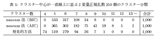
-(Quoted from the paper) Accuracy comparison when the number of correct clusters is 5 ――The number of correct clusters is larger when evaluated by BIC than by AIC. --AIC tends to produce a relatively large number of clusters --The result of the discovery method (the method of manually specifying the k number with k-means) is close to the result of BIC (if it is the same as the result obtained manually, x-mean that does it automatically is better! )
Differences in logic between the two papers
Outline of the original paper of 1
--Implicitly assume that all clusters have the same distribution of data
Summary of 2 improved logic papers
――The center of gravity should be different depending on the size of the cluster, so the logic is made to estimate that as well.
Other blog posts about x-means: -Implemented x-means method in Python -x-means (In the OpenCV sample, an article in which color reduction / image division processing using k-means is replaced with x-means. ) -x-means method -K-means method in R and its extension 2 x-means edition | Sabotage prohibited diary
X-means script in Python
Implemented x-means method in Python [Gist code] Copy / yasaichi / 254a060eff56a3b3b858)
# -*- coding: utf-8 -*-
import numpy as np
from scipy import stats
from sklearn.cluster import KMeans
import matplotlib.pyplot as plt
from IPython.display import display, HTML #For Jupyter notebook
%matplotlib inline
class XMeans:
    """
    x-Class that does the means method
    """

    def __init__(self, k_init = 2, **k_means_args):
        """
        k_init : The initial number of clusters applied to KMeans()
        """
        self.k_init = k_init
        self.k_means_args = k_means_args

    def fit(self, X):
        """
        x-Cluster data X using means method
        X : array-like or sparse matrix, shape=(n_samples, n_features)
        """
        self.__clusters = []

        clusters = self.Cluster.build(X, KMeans(self.k_init, **self.k_means_args).fit(X))
        self.__recursively_split(clusters)

        self.labels_ = np.empty(X.shape[0], dtype = np.intp)
        for i, c in enumerate(self.__clusters):
            self.labels_[c.index] = i

        self.cluster_centers_ = np.array([c.center for c in self.__clusters])
        self.cluster_log_likelihoods_ = np.array([c.log_likelihood() for c in self.__clusters])
        self.cluster_sizes_ = np.array([c.size for c in self.__clusters])

        return self

    def __recursively_split(self, clusters):
        """
Recursively split the argument clusters
        clusters : list-like object, which contains instances of 'XMeans.Cluster'
        'XMeans.Cluster'List type object containing an instance of
        """
        for cluster in clusters:
            if cluster.size <= 3:
                self.__clusters.append(cluster)
                continue

            k_means = KMeans(2, **self.k_means_args).fit(cluster.data)
            c1, c2 = self.Cluster.build(cluster.data, k_means, cluster.index)

            beta = np.linalg.norm(c1.center - c2.center) / np.sqrt(np.linalg.det(c1.cov) + np.linalg.det(c2.cov))
            alpha = 0.5 / stats.norm.cdf(beta)
            bic = -2 * (cluster.size * np.log(alpha) + c1.log_likelihood() + c2.log_likelihood()) + 2 * cluster.df * np.log(cluster.size)

            if bic < cluster.bic():
                self.__recursively_split([c1, c2])
            else:
                self.__clusters.append(cluster)

    class Cluster:
        """
        k-A class that has information about clusters generated by the means method and calculates likelihood and BIC.
        """

        @classmethod
        def build(cls, X, k_means, index = None):
            if index == None:
                index = np.array(range(0, X.shape[0]))
            labels = range(0, k_means.get_params()["n_clusters"])

            return tuple(cls(X, index, k_means, label) for label in labels)

        # index:A vector indicating which line of the original data the sample in each row of X belongs to
        def __init__(self, X, index, k_means, label):
            self.data = X[k_means.labels_ == label]
            self.index = index[k_means.labels_ == label]
            self.size = self.data.shape[0]
            self.df = self.data.shape[1] * (self.data.shape[1] + 3) / 2
            self.center = k_means.cluster_centers_[label]
            self.cov = np.cov(self.data.T)

        def log_likelihood(self):
            return sum(stats.multivariate_normal.logpdf(x, self.center, self.cov) for x in self.data)

        def bic(self):
            return -2 * self.log_likelihood() + self.df * np.log(self.size)
if __name__ == "__main__":
    import matplotlib.pyplot as plt

    #Data preparation
    x = np.array([np.random.normal(loc, 0.1, 20) for loc in np.repeat([1,2], 2)]).flatten() #Generate 80 random numbers
    y = np.array([np.random.normal(loc, 0.1, 20) for loc in np.tile([1,2], 2)]).flatten() #Generate 80 random numbers

    #Performing clustering
    x_means = XMeans(random_state = 1).fit(np.c_[x,y])
    print(x_means.labels_)
    print(x_means.cluster_centers_)
    print(x_means.cluster_log_likelihoods_)
    print(x_means.cluster_sizes_)

    #Plot the results
    plt.rcParams["font.family"] = "Hiragino Kaku Gothic Pro"
    plt.scatter(x, y, c = x_means.labels_, s = 30)
    plt.scatter(x_means.cluster_centers_[:,0], x_means.cluster_centers_[:,1], c = "r", marker = "+", s = 100)
    plt.xlim(0, 3)
    plt.ylim(0, 3)
    plt.title("x-means_test1")
    plt.legend()
    plt.grid()
    plt.show()
    # plt.savefig("clustering.png ", dpi = 200)
[1 1 1 1 1 1 1 1 1 1 1 1 1 1 1 1 1 1 1 1 0 0 0 0 0 0 0 0 0 0 0 0 0 0 0 0 0
 0 0 0 3 3 3 3 3 3 3 3 3 3 3 3 3 3 3 3 3 3 3 3 2 2 2 2 2 2 2 2 2 2 2 2 2 2
 2 2 2 2 2 2]
[[ 1.01854145  2.00982242]
 [ 1.00199794  1.02110352]
 [ 2.00022392  2.00435037]
 [ 2.04408807  1.0518478 ]]
[ 42.91288569  44.48049658  37.32131967  29.6422041 ]
[20 20 20 20]
⇒ X-means was performed on the data of 4 clusters, and it was certainly divided into 4 clusters without specifying an explicit k number!
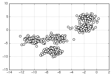
Try clustering data that looks a bit more like that
(The number of clusters specified at the time of generation is 5)
from sklearn.datasets import make_blobs
X, y = make_blobs(n_samples=500,
                  n_features=2,
                  centers=5,
                  cluster_std=0.8,
                  center_box=(-10.0, 10.0),
                  shuffle=True,
                  random_state=1)  # For reproducibility

x =X[:,0]
y =X[:,1]
X=np.c_[x,y]

plt.scatter(x,y,c='white',marker='o',s=50)
plt.grid()
plt.show()
if __name__ == "__main__":
    import matplotlib.pyplot as plt

    #Performing clustering
    x_means = XMeans(random_state = 1).fit(np.c_[X])

    #Plot the results
    plt.rcParams["font.family"] = "Hiragino Kaku Gothic Pro"
    plt.scatter(x, y, c = x_means.labels_, s = 30)
    plt.scatter(x_means.cluster_centers_[:,0], x_means.cluster_centers_[:,1], c = "r", marker = "*", s = 250)
    plt.title("x-means_test2")
    plt.grid()
    plt.show()

⇒ This is also divided properly!
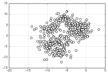
Try clustering more moody data
(The number of clusters specified at the time of generation is 8)
from sklearn.datasets import make_blobs
X, y = make_blobs(n_samples=500,
                  n_features=2,
                  centers=8,
                  cluster_std=1.5,
                  center_box=(-10.0, 10.0),
                  shuffle=True,
                  random_state=1)  # For reproducibility

x =X[:,0]
y =X[:,1]
X=np.c_[x,y]

plt.scatter(X[:,0],X[:,1],c='white',marker='o',s=50)
plt.grid()
plt.show()
if __name__ == "__main__":
    import matplotlib.pyplot as plt

    #Performing clustering
    x_means = XMeans(random_state = 1).fit(np.c_[X])

    #Plot the results
    plt.rcParams["font.family"] = "Hiragino Kaku Gothic Pro"
    plt.scatter(x, y, c = x_means.labels_, s = 30)
    plt.scatter(x_means.cluster_centers_[:,0], x_means.cluster_centers_[:,1], c = "r", marker = "*", s = 250)
    plt.title("x-means_test3")
    plt.grid()
    plt.show()

=> In x-means automatic clustering, the optimum number of clusters is calculated as "5". It feels like it's divided.
I will try to write an elbow book again without sexual discipline
See Previous article for how to read the elbow diagram. (Output the sum of squared errors in clusters 1 to 10 together)
distortions = []

for i  in range(1,11):                # 1~Calculate up to 10 clusters at once
    km = KMeans(n_clusters=i,         #Number of clusters
                init='k-means++',     # k-means++Select cluster center by law
                n_init=10,            #K with different initial values of centroids-means execution count default: '10'Select the model with the smaller SSE value as the final model
                max_iter=300,         # k-means Maximum number of iterations inside the algorithm default: '300'
                random_state=0)       #State of the random number generator used to initialize the centroid
    km.fit(X)                         #Perform clustering calculations
    distortions.append(km.inertia_)   # km.fit and km.inertia_Is sought
    y_km = km.fit_predict(X)

plt.plot(range(1,11),distortions,marker='o')
plt.xlabel('Number of clusters')
plt.ylabel('Distortion')
plt.show()

=> It is still difficult to judge the optimum number of clusters as "5" from this figure.
I will try to write a silhouette book again without sexual discipline
See Previous article for how to read the silhouette diagram. (Silhouette diagrams of clusters 3 to 8 are output together)
Borrow the code from scikit-learn official page Partially rewritten)
km = KMeans(n_clusters=5,       #Number of clusters
            init='k-means++',   # k-means++Select cluster center by law
            n_init=10,          #K with different initial values of centroids-means execution count default: '10'Select the model with the smaller SSE value as the final model
            max_iter=300,       # k-means Maximum number of iterations inside the algorithm default: '300'
            random_state=0)     #State of the random number generator used to initialize the centroid
y_km = km.fit_predict(X)
from __future__ import print_function

from sklearn.datasets import make_blobs
from sklearn.cluster import KMeans
from sklearn.metrics import silhouette_samples, silhouette_score

import matplotlib.pyplot as plt
import matplotlib.cm as cm
import numpy as np

print(__doc__)

# Generating the sample data from make_blobs

X, y = make_blobs(n_samples=500,
                  n_features=2,
                  centers=8,
                  cluster_std=1.5,
                  center_box=(-10.0, 10.0),
                  shuffle=True,
                  random_state=1)  # For reproducibility

range_n_clusters = [3, 4, 5, 6, 7, 8]

for n_clusters in range_n_clusters:
    # Create a subplot with 1 row and 2 columns
    fig, (ax1, ax2) = plt.subplots(1, 2)
    fig.set_size_inches(18, 7)

    # The 1st subplot is the silhouette plot
    # The silhouette coefficient can range from -1, 1 but in this example all
    # lie within [-0.1, 1]
    ax1.set_xlim([-0.1, 1])
    # The (n_clusters+1)*10 is for inserting blank space between silhouette
    # plots of individual clusters, to demarcate them clearly.
    ax1.set_ylim([0, len(X) + (n_clusters + 1) * 10])

    # Initialize the clusterer with n_clusters value and a random generator
    # seed of 10 for reproducibility.
    clusterer = KMeans(n_clusters=n_clusters, random_state=1)
    cluster_labels = clusterer.fit_predict(X)

    # The silhouette_score gives the average value for all the samples.
    # This gives a perspective into the density and separation of the formed
    # clusters
    silhouette_avg = silhouette_score(X, cluster_labels)
    print("For n_clusters =", n_clusters,
          "The average silhouette_score is :", silhouette_avg)

    # Compute the silhouette scores for each sample
    sample_silhouette_values = silhouette_samples(X, cluster_labels,metric='euclidean')

    y_lower = 10
    for i in range(n_clusters):
        # Aggregate the silhouette scores for samples belonging to
        # cluster i, and sort them
        ith_cluster_silhouette_values = \
            sample_silhouette_values[cluster_labels == i]

        ith_cluster_silhouette_values.sort()

        size_cluster_i = ith_cluster_silhouette_values.shape[0]
        y_upper = y_lower + size_cluster_i

        color = cm.spectral(float(i) / n_clusters)
        ax1.fill_betweenx(np.arange(y_lower, y_upper),
                          0, ith_cluster_silhouette_values,
                          facecolor=color, edgecolor=color, alpha=0.7)

        # Label the silhouette plots with their cluster numbers at the middle
        ax1.text(-0.05, y_lower + 0.5 * size_cluster_i, str(i))

        # Compute the new y_lower for next plot
        y_lower = y_upper + 10  # 10 for the 0 samples

    ax1.set_title("The silhouette plot for the various clusters.")
    ax1.set_xlabel("The silhouette coefficient values")
    ax1.set_ylabel("Cluster label")

    # The vertical line for average silhoutte score of all the values
    ax1.axvline(x=silhouette_avg, color="red", linestyle="--")

    ax1.set_yticks([])  # Clear the yaxis labels / ticks
    ax1.set_xticks([-0.1, 0, 0.2, 0.4, 0.6, 0.8, 1])

    # 2nd Plot showing the actual clusters formed
    colors = cm.spectral(cluster_labels.astype(float) / n_clusters)
    ax2.scatter(X[:, 0], X[:, 1], marker='.', s=30, lw=0, alpha=0.7,
                c=colors)

    # Labeling the clusters
    centers = clusterer.cluster_centers_
    # Draw white circles at cluster centers
    ax2.scatter(centers[:, 0], centers[:, 1],
                marker='o', c="white", alpha=1, s=200)

    for i, c in enumerate(centers):
        ax2.scatter(c[0], c[1], marker='$%d$' % i, alpha=1, s=100)

    ax2.set_title("The visualization of the clustered data.")
    ax2.set_xlabel("Feature space for the 1st feature")
    ax2.set_ylabel("Feature space for the 2nd feature")

    plt.suptitle(("Silhouette analysis for KMeans clustering on sample data "
                  "with n_clusters = %d" % n_clusters),
                 fontsize=14, fontweight='bold')
    plt.grid()
    plt.show()
Automatically created module for IPython interactive environment
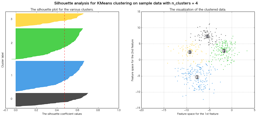
For n_clusters = 3 The average silhouette_score is : 0.500273979793

For n_clusters = 4 The average silhouette_score is : 0.473805434223
For n_clusters = 5 The average silhouette_score is : 0.451524016461

For n_clusters = 6 The average silhouette_score is : 0.428239776719

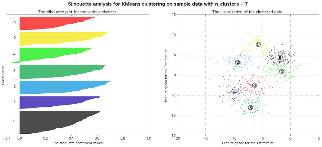
For n_clusters = 7 The average silhouette_score is : 0.427688325647
For n_clusters = 8 The average silhouette_score is : 0.409792863353

=> Evaluation of silhouette diagram Legally, it seems that 7 or 8 clusters are good.
Conclusion
――X-means certainly seems to cluster nicely ――However, there is no way to "match" the number of clusters, and do you feel that you will use it to "get a" guideline "for the optimal number of clusters?" ――It is still difficult to get an estimate of the optimum number of clusters from the elbow diagram ...? --Similar to the silhouette method ...
⇒ After all, does it feel like selecting a cluster that has obtained easy-to-interpret results according to the purpose of clustering to some extent?
Appendix (I researched various things to understand the contents)
Let's examine the logic of the x-means method! → I don't know the Bayesian Information Criterion (BIC) → I don't know AIC properly in the first place → Likelihood is what after all? → There is a Bayesian estimation other than the maximum likelihood estimation to find the likelihood ... Endlessly continuing from there yak shaving
"Acutally, my whole life is just one big yak shaving exercise." - Joi Ito
Akaike's Information Criterion: AIC (Akaike's Information Criterion)
Indicator for selecting a model with the optimum number of parameters
――The model created for a certain data can improve the goodness of fit with the existing data by increasing the parameters, but it falls into overfitting. ――It is necessary to reduce the number of modeling parameters in order not to fall into overfitting, but it is a difficult problem to actually reduce the number. --Calculating the AIC with the model and showing the ** minimum value ** will often make a good model selection ――Since AIC is composed of the log-likelihood of the model and the number of parameters, the trade-off between accuracy and complexity can be described nicely.
--The first term of the equation represents the good fit to the model, and the second term represents the penalty for the complexity of the model. --In the second term, the smaller the number of parameters, the more the overfitting problem can be avoided, so it works better for the model with the smaller number of parameters. ――Even if the fit is good, a messy and complicated model is not preferable, so an index that fits well and is aimed at a simple model ――It can be said that a good model can generally be selected by calculating the AIC for all the target models and selecting the smallest model.
reference:
- Akaike Information Ctiteriion | wikipedia -Time Series Analysis II-Evaluation and Future Prediction of ARMA Model (Autoregressive-moving Average Model) | @IT
Bayesian Information Criterion (BIC)
--In many cases, good model selection can be made if BIC shows the minimum value. --Compared to AIC, an index that also considers the sample size as a penalty for the complexity of the model in Section 2. ――Unlike AIC, selection by this criterion has consistency (a large number of samples results in a true order).
reference:
Bayesian Information Criterion | wikipedia
Difference between AIC and BIC
--Difference in purpose --Use AIC if model selection is used to improve prediction accuracy --Use BIC if you want to know the structure from which the data is generated
--Mathematical difference --Penalty item in paragraph 2 ――In AIC, when the sample size is large regardless of the sample size, the specific gravity of the first term becomes large and a complicated model tends to be selected. --In BIC, the sample size is taken into consideration in the penalties, so a simpler model than AIC tends to be selected.
--Difference in model parameter estimation strategy --AIC determines the maximum value of the likelihood function by maximum likelihood estimation --BIC determines the maximum value of the likelihood function by Bayesian estimation
――However, there is no consensus that it must be used in this way.
reference: -Akaike Information Criterion AIC and Bayesian Information Criterion BIC | Tell me! Goo -[Bayesian Information Criterion and Its Development-Overview- | ALBERT Official Blog](http://blog.albert2005.co.jp/2016/04/19/%E3%83%99%E3%82%A4% E3% 82% BA% E6% 83% 85% E5% A0% B1% E9% 87% 8F% E8% A6% 8F% E6% BA% 96% E5% 8F% 8A% E3% 81% B3% E3% 81% 9D% E3% 81% AE% E7% 99% BA% E5% B1% 95-% EF% BD% 9E% E6% A6% 82% E8% AA% AC% E7% B7% A8% EF% BD % 9E /)
Likelihood review
Review of "What was the likelihood in the first place?"
The likelihood of a model when considered from the obtained data is called likelihood. Source
The basic concept of the likelihood function is to answer the question ** "After sampling and observing the data, what parameters did the data originally come from?" ** is. Source
Likelihood is just like probability. However, the way of thinking is different. For probability, the parameters are fixed and the data change, but for likelihood, the data are fixed and the parameters change. Source
reference:
-[Statistics] What is likelihood? Let's explain graphically. | Qiita
-Likelihood and maximum likelihood estimation method | Sunny side up!
What is maximum likelihood estimation?
When the likelihood is maximum = Know the parameters (mean and variance in the case of Gaussian distribution) of the model you want to estimate (probability distribution: basically Gaussian distribution)
Difference between maximum likelihood estimation and Bayesian estimation
| is what? | Method | In other words | |
|---|---|---|---|
| Maximum likelihood estimation | Maximize the likelihoodHow to calculate the parameters | Likelihood onlyEstimate the parameters with (do not consider prior probabilities) | Estimate the parameters using only the probabilities of the data just acquired |
| Bayesian inference | Maximize posterior probabilitiesHow to calculate the parameters | Prior probabilities and likelihoodsEstimate parameters using both | Estimate parameters using prior and posterior probabilities as well as the data just acquired |
reference:
-Who is the likelihood? | MyEnigma
-Difference between Bayesian estimation and maximum likelihood estimation | Tech Tips
Which should I use, maximum likelihood estimation or Bayesian estimation?
-(Roughly speaking) Both are basically the same --The biggest difference is ** whether to consider "prior probabilities" ** --Maximum likelihood estimation does not consider prior probabilities (= it can be said that a uniform distribution is assumed). In other words, the start is when there is no information. --If the prior probabilities are not uniform, the results of maximum likelihood estimation and Bayesian estimation are different. --In Bayesian estimation, if the optimum prior probability can be set, more accurate estimation can be performed. --Bayesian inference is an estimate that makes use of more information. --The prior probability setting tends to be subjective. This seems to be the center of the controversy between maximum likelihood and Bayesian --In particular, if there is no prediction in advance or the optimum prior distribution is not known, a prior distribution called "no information distribution" is used (many programs default to no information distribution).
Reference: Difference between conventional estimation method and Bayesian estimation method | Sunny side up!
About Bayesian inference
A typical indicator of the goodness of fit of Bayesian estimation is ** Bayes factor (BF) ** --BF represents the ** likelihood ratio ** of the two models --BF can be approximated to BIC (Bayesian Information Criterion) --Difference in BIC between the two models ≒ 2 times the logarithm of BF (* Note that they are different just by approximating)
Reference: Bayes factor and model selection | SlideShare
Bayes factor criteria
| BF | 2logBF (≒BIC) | Judgment for M1 compared to M0 |
|---|---|---|
| BF<1 | 2logBF<0 | M0 is better |
| 1<BF<3 | 0<2logBF<2 | M1 is barely better |
| 3<BF<12 | 2<2logBF<5 | M1 is better (Positive) |
| 12<BF<150 | 5<2logBF<10 | M1 is much better (Strong) |
| 150<BF | 10<2logBF | M1 is much better (Very Strong) |
Advantages and problems of using Bayes factor for model evaluation
■ Merit
--Release from the curse of the null hypothesis --The traditional test has a composition of "null hypothesis" and "alternative hypothesis". --Bayes factor, but just compare "two independent models (hypotheses)" --There is no need to have a "null hypothesis"
--Free from the curse of the normal distribution --Bayesian equation incorporates prior distribution ―― “The prior distribution does not have to be a normal distribution” → It can be examined by applying a more flexible statistical model ・ ・ ・ Bayesian estimation is used
■ Problems
--Bayes factor is the "likelihood ratio" of the two models ――The magnitude of the numerical value can only be "Compare the two and which is better" ――It is good to calculate multiple indicators and think in total --Calculation is difficult ――It becomes difficult due to the increase of parameters and prior distribution.
For other advantages and disadvantages of Bayesian estimation, see here.
Others that serve as an index (reference) for selecting the most suitable model
--Deviance Information Criterion (DIC) --Post-mortem P-value
--The problem with indicators such as AIC and BIC is that they cannot be applied to singular models that include latent variables. ――It seems that there is also an amount of information called FIC (Factorized Information Criterion) and FAB (Factorized Asymptotic Bayesian inference) to deal with these.
Reference: [Paper] A brief summary of heterogeneous blended learning | Feces Net Benkei
Recommended Posts