Implemented Perceptron learning rules in Python
About this post
I implemented the learning rule of Perceptron, which is one of the methods for determining the discrimination boundary for linearly separable data groups, in Python without using a library. Since I am a beginner in both Python and machine learning, please point out the bad points.
For "Widrow-Hoff learning rules" that are compared alongside "Perceptron learning rules", see "Implementing Widrow-Hoff learning rules in Python" [http: / /qiita.com/s-kiriki/items/6a90beede4c139558bcc).
Perceptron's theory of learning rules
An overview of Perceptron's learning rules and mathematical formulas are summarized in the slides below (starting in the middle of the slide).
https://speakerdeck.com/kirikisinya/xin-zhe-renaiprmlmian-qiang-hui-at-ban-zang-men-number-2
Implementation
In the case of one dimension
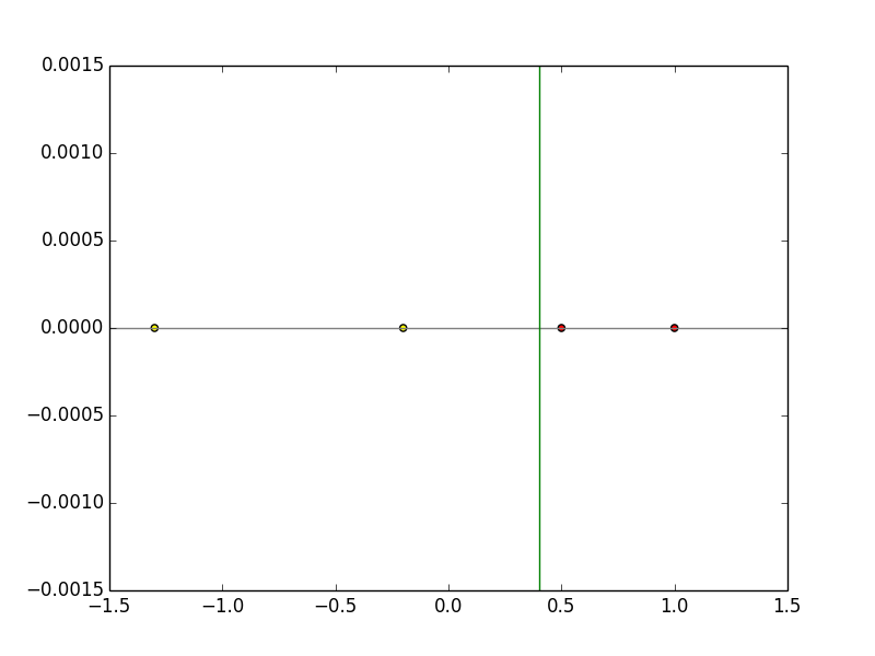
Find the separation boundary line of linearly separable training data that exists on one dimension as shown in the figure below and belongs to one of the two classes.

As a point of implementation,
- The initial weight vector is
w = (0.2,0.3)and the learning coefficient isρ = 0.5. - The convergence test of the separation boundary was not performed, and the weight vector correction (learning) was repeated a sufficient number of times (100 times) (I think it's not really good, but I thought it would be good to let the machine do a lot of work. .)
The actual code looks like this:
# coding: UTF-8
#Implementation example of one-dimensional perceptron learning rules
import numpy as np
import matplotlib.pyplot as plt

def train(wvec, xvec, is_c1):
    low = 0.5#Learning coefficient
    if (np.dot(wvec,xvec) > 0) != is_c1:
        if is_c1:
            wvec_new = wvec + low*xvec
        else:
            wvec_new = wvec - low*xvec
        return wvec_new
    else:
        return wvec

if __name__ == '__main__':

    data = np.array([[1.0, 1],[0.5, 1],[-0.2, 2],[-1.3, 2]])#Data group

    features = data[:,0].reshape(data[:,0].size,1)#Feature vector
    labels = data[:,1]#Class (this time c1=1,c2=2)
    wvec = np.array([0.2, 0.3])#Initial weight vector
    is_c1s = (labels == 1)#Array of boolean whether c1

    xvecs = np.c_[np.ones(features.size), features]#xvec[0] = 1

    loop = 100
    for j in range(loop):
        for xvec, is_c1 in zip(xvecs, is_c1s):
            wvec = train(wvec, xvec, is_c1)

    print wvec
    print -(wvec[0]/wvec[1])

    #Graph depiction
    plt.axhline(y=0, c='gray')
    plt.scatter(features[is_c1s], np.zeros(features[is_c1s].size), c='red', marker="o")
    plt.scatter(features[~is_c1s], np.zeros(features[~is_c1s].size), c='yellow', marker="o")
    #Separation border
    plt.axvline(x=-(wvec[0]/wvec[1]), c='green')
    plt.show()
The weight vector after training is w = (-0.3, 0.75).
Substituting this into the formula wx = 0, the discriminant function becomes x = 0.4, and it can be seen that the linear separation is successfully performed by learning as shown in the figure below.

In the case of 2D
As shown in the figure below (image), find the separation boundary line of linearly separable training data that exists in two dimensions and belongs to one of the two classes.

As a point of implementation,
- Use
np.random.randto generate two linearly separable classes of data - The initial weight vector is
w = (2, -1,3)and the learning coefficient isρ = 0.5. - As in the case of one dimension, the convergence test of the separation boundary was not performed, and the weight vector correction (learning) was repeated a sufficient number of times (100 times).
The actual code looks like this:
# coding: UTF-8
#Implementation example of 2D perceptron learning rules
import numpy as np
import matplotlib.pyplot as plt
import sys

def train(wvec, xvec, label):
    low = 0.5#Learning coefficient
    if (np.dot(wvec,xvec) * label < 0):
        wvec_new = wvec + label*low*xvec
        return wvec_new
    else:
        return wvec

if __name__ == '__main__':

    train_num = 100#Number of training data

    #Class 1 learning data
    x1_1=np.random.rand(train_num/2) * 5 + 1 #x component
    x1_2=np.random.rand(int(train_num/2)) * 5 + 1 #y component
    label_x1 = np.ones(train_num/2) #Label (all 1)

    #Class 2 learning data
    x2_1=(np.random.rand(train_num/2) * 5 + 1) * -1 #x component
    x2_2=(np.random.rand(train_num/2) * 5 + 1) * -1 #y component
    label_x2 = np.ones(train_num/2) * -1 #Label (all-1)

    x0=np.ones(train_num/2) #x0 is always 1
    x1=np.c_[x0, x1_1, x1_2]
    x2=np.c_[x0, x2_1, x2_2]

    xvecs=np.r_[x1, x2]
    labels = np.r_[label_x1, label_x2]

    wvec = np.array([2,-1,3])#Initial weight vector Determine appropriately

    loop = 100
    for j in range(loop):
        for xvec, label in zip(xvecs, labels):
            wvec = train(wvec, xvec, label)

    print wvec

    plt.scatter(x1[:,1], x1[:,2], c='red', marker="o")
    plt.scatter(x2[:,1], x2[:,2], c='yellow', marker="o")
    #Separation border
    x_fig = np.array(range(-8,8))
    y_fig = -(wvec[1]/wvec[2])*x_fig - (wvec[0]/wvec[2])

    plt.plot(x_fig,y_fig)
    plt.show()
Since the training data is randomly generated, the weight vector and discriminant function after training are different each time, As an example of the actual execution result, it is shown in the figure below, and it can be seen that the linear separation is successfully performed by learning.

Recommended Posts