Multivariate LSTM with Keras
I often see univariate time series in keras, but since multiple factors are involved when forecasting stock prices and sales, this time I tried to forecast using multiple time series data. ..
Source introduction
code
Based on the code introduced in "MACHINE LEARNING MASTERY", it supports multivariate. Time Series Prediction with LSTM Recurrent Neural Networks in Python with Keras
Click here for the full code that can be seen on jupyter https://github.com/tizuo/keras/blob/master/LSTM%20with%20multi%20variables.ipynb
data
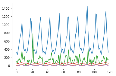
Sample data is borrowed from the following. Predict the leftmost ice_sales. How to sell ice cream
| ice_sales | year | month | avg_temp | total_rain | humidity | num_day_over25deg |
|---|---|---|---|---|---|---|
| 331 | 2003 | 1 | 9.3 | 101 | 46 | 0 |
| 268 | 2003 | 2 | 9.9 | 53.5 | 52 | 0 |
| 365 | 2003 | 3 | 12.7 | 159.5 | 49 | 0 |
| 492 | 2003 | 4 | 19.2 | 121 | 61 | 3 |
| 632 | 2003 | 5 | 22.4 | 172.5 | 65 | 7 |
| 730 | 2003 | 6 | 26.6 | 85 | 69 | 21 |
| 821 | 2003 | 7 | 26 | 187.5 | 75 | 21 |

Data standardization
Standardize the data. It was explained that LSTMs are sensitive and the numbers they handle must be standardized.
python
scaler = MinMaxScaler(feature_range=(0, 1))
dataset = scaler.fit_transform(dataset)
Separate test data
This time, we will predict the data of the latter half 1/3, so we will separate it from the one for learning.
python
train_size = int(len(dataset) * 0.67)
test_size = len(dataset) - train_size
train, test = dataset[0:train_size,:], dataset[train_size:len(dataset),:]
Data shaping
Since we will learn the value of the next month using the value up to 3 months ago, format it as follows. Create variables that use this and store them in the data for one time point.
| Y | 3 months ago | 2 months ago | 1 month ago |
|---|---|---|---|
| January value | October value | 1January value | December value |
| February value | November value | 1February value | January value |
| March value | December value | January value | February value |
This time, we consider it as one set per year, and lookback creates data with 12.
python
def create_dataset(dataset, look_back=1):
    dataX, dataY = [], []
    for i in range(len(dataset)-look_back-1):
        xset = []
        for j in range(dataset.shape[1]):
            a = dataset[i:(i+look_back), j]
            xset.append(a)
        dataY.append(dataset[i + look_back, 0])
        dataX.append(xset)
    return numpy.array(dataX), numpy.array(dataY)

look_back = 12
trainX, trainY = create_dataset(train, look_back)
testX, testY = create_dataset(test, look_back)
Convert this data to a format accepted by keras LSTMs. [Number of rows]> [Number of variables]> [Number of columns (number of lookups)]
python
trainX = numpy.reshape(trainX, (trainX.shape[0], trainX.shape[1], trainX.shape[2]))
testX = numpy.reshape(testX, (testX.shape[0], testX.shape[1], testX.shape[2]))
Modeling
input_shape contains the number of variables and the number of lookups. The number of outputs is set to 4 as shown in the sample without considering it.
python
model = Sequential()
model.add(LSTM(4, input_shape=(testX.shape[1], look_back)))
model.add(Dense(1))
model.compile(loss='mean_squared_error', optimizer='adam')
model.fit(trainX, trainY, epochs=1000, batch_size=1, verbose=2)
Verification
The prediction is the same as usual.
python
trainPredict = model.predict(trainX)
testPredict = model.predict(testX)
After this, return Y to the unstandardized number. Since the scaler is not accepted unless it has the same shape as the original dataset, the value is padded with 0s for the number of columns that existed. Please let me know if there is a smarter way.
python
pad_col = numpy.zeros(dataset.shape[1]-1)
def pad_array(val):
    return numpy.array([numpy.insert(pad_col, 0, x) for x in val])

trainPredict = scaler.inverse_transform(pad_array(trainPredict))
trainY = scaler.inverse_transform(pad_array(trainY))
testPredict = scaler.inverse_transform(pad_array(testPredict))
testY = scaler.inverse_transform(pad_array(testY))
Finally get the standard deviation.
python
trainScore = math.sqrt(mean_squared_error(trainY[:,0], trainPredict[:,0]))
print('Train Score: %.2f RMSE' % (trainScore))
testScore = math.sqrt(mean_squared_error(testY[:,0], testPredict[:,0]))
print('Test Score: %.2f RMSE' % (testScore))
After changing the number of variables, it became as follows. Of course, you have to choose the variable to throw.
| A model learned only from ice cream sales | Ice cream and 25 degrees or more days | All | |
|---|---|---|---|
| Train Score | 30.20 RMSE | 15.19 RMSE | 8.44 RMSE |
| Test Score | 111.97 RMSE | 108.09 RMSE | 112.90 RMSE |

Recommended Posts