Deep Learning

Deep Learing

perceptron

background

This program was devised in 1957 by a researcher named Rosenblatt in the United States. Perceptron is the algorithm that is the origin of neural networks.

What is Perceptron?

It receives multiple signals as input and outputs one signal. The perceptron signal is "1 or 0". The perceptron that receives the two signals as inputs is as follows.

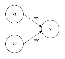
Input signal: x1, x2 Output signal: y Weights: w1, w2 When the input signal is sent to the neuron, each is multiplied by a unique weight, and 1 is output only when the sum of the input signals exceeds the limit value (threshold value, θ).

f(x) = \left\{
\begin{array}{ll}
0 & (w1x1 + w2x2 \leq θ) \\
1 & (w1x1 + w2x2 \gt θ)
\end{array}
\right.

Implementation of perceptron

Taking AND gate as an example ...

def AND(x1,x2):
    w1,w2,theta = 0.5,0.5,0.7
    tmp = x1*w1 + x2*w2
    if tmp <= theta:
        return 0
    elif tmp > theta:
        return 1

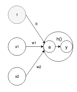
Introducing bias

Transform the above equation with θ as -b

f(x) = \left\{
\begin{array}{ll}
0 & (b + w1x1 + w2x2 \leq 0) \\
1 & (b + w1x1 + w2x2 \gt 0)
\end{array}
\right.

The AND gate looks like this

import numpy as np
def AND(x1,x2):
    x = np.array([x1,x2])
    w = np.array([0.5,0.5])
    b = -0.7
    tmp = np.sum(w*x) + b
    if tmp <= 0:
        return 0
    else:
        return 1

The NAND gate looks like this

import numpy as np
def AND(x1,x2):
    x = np.array([x1,x2])
    w = np.array([-0.5,-0.5])
    b = 0.7
    tmp = np.sum(w*x) + b
    if tmp <= 0:
        return 0
    else:
        return 1

The OR gate looks like this

import numpy as np
def AND(x1, x2):
    x = np.array([x1, x2])
    w = np.array([0.5, 0.5])
    b = -0.2
    tmp = np.sum(w * x) + b
    if tmp <= 0:
        return 0
    else:
        return 1

Difference in work

Weight => Control the importance of the input signal Bias => Controls ease of ignition

The limits of perceptron

Perceptons cannot represent XOR gates. However, it can be expressed by ** stacking layers **.

def XOR(x1,x2):
    s1 = NAND(x1,x2)
    s2 = OR(x1,x2)
    y = AND(s1,s2)
    return y

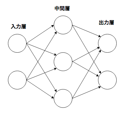
neural network

It has the property that appropriate weight parameters can be automatically learned from the data.

Activation function

The activation function is a function that converts the sum of input signals into an output signal. In neural networks, it is necessary to use nonlinear functions.

a = b + w1x1 + w2x2 \\
y = h(a)

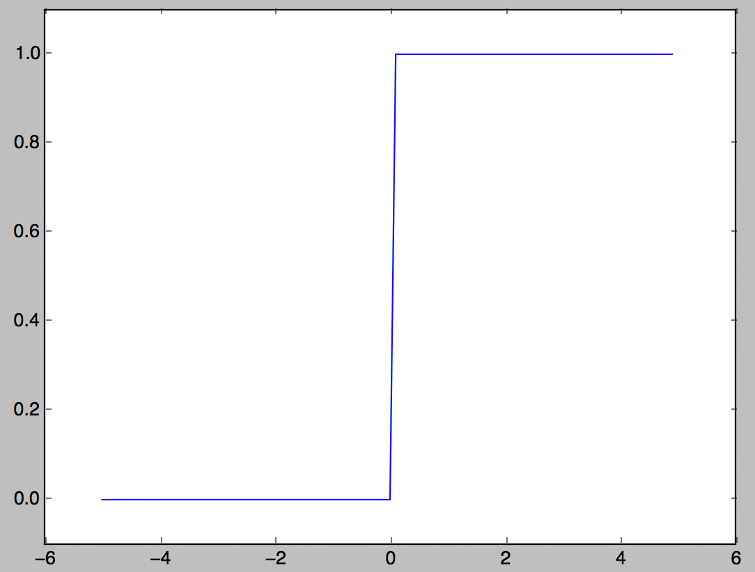
Step function

One of the activation functions that outputs 1 when the input exceeds 0, and outputs 0 otherwise.

import numpy as np
import matplotlib.pylab as plt
def step_function(x):
    y = x > 0
    return y.astype(np.int)

x = np.arange(-5.0,5.0,0.1)
y = step_function(x)
plt.plot(x,y)
plt.ylim(-0.1,1.1)
plt.show()

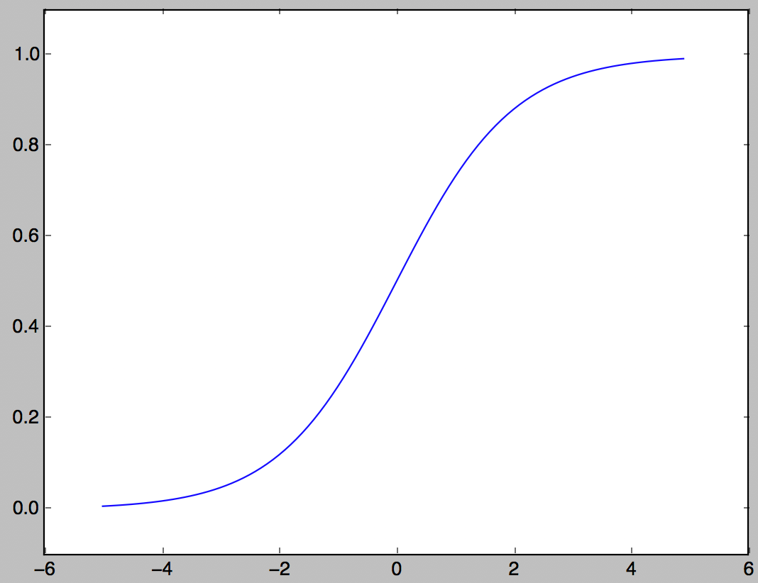
Sigmoid function

One of the activation functions often used in neural networks.

h(x) = \frac{1}{1+e^{-x}}

import numpy as np
import matplotlib.pylab as plt
def sigmoid(x):
    return 1/(1+np.exp(-x))

x = np.arange(-5.0,5.0,0.1)
y = sigmoid(x)
plt.plot(x,y)
plt.ylim(-0.1,1.1)
plt.show()

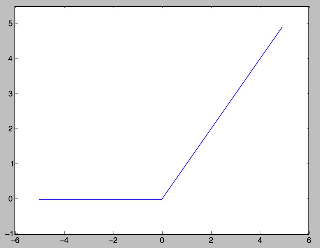
ReLU function

An activation function that is often used these days. If the input exceeds 0, the input is output as it is, and if it is 0 or less, 0 is output.

h(x) = \left\{
\begin{array}{ll}
x & (x \gt 0) \\
0 & (x \leq 0)
\end{array}
\right.

import numpy as np
import matplotlib.pylab as plt
def relu(x):
    return np.maximum(0, x)

x = np.arange(-5.0,5.0,0.1)
y = relu(x)
plt.plot(x,y)
plt.ylim(-1.0,5.5)
plt.show()

Implementation of 3-layer neural network

#Define a number
def init_network():
    network = {}
    network['W1'] = np.array([[0.1, 0.3, 0.5], [0.2, 0.4, 0.6]])
    network['b1'] = np.array([0.1, 0.2, 0.3])
    network['W2'] = np.array([[0.1, 0.4], [0.2, 0.5], [0.3, 0.6]])
    network['b2'] = np.array([0.1, 0.2])
    network['W3'] = np.array([[0.1, 0.3], [0.2, 0.4]])
    network['b3'] = np.array([0.1, 0.2])

    return network

#Function to calculate up to the output layer
def forward(network, x):
    W1, W2, W3 = network['W1'], network['W2'], network['W3']
    b1, b2, b3 = network['b1'], network['b2'], network['b3']

    a1 = np.dot(x, W1) + b1
    z1 = sigmoid(a1)
    a2 = np.dot(z1, W2) + b2
    z2 = sigmoid(a2)
    a3 = np.dot(z2, W3) + b3
    y = identity_function(a3)

    return y

#Implementation
network = init_network()
x = np.array([1.0, 0.5])
y = forward(network, x)

Softmax function

Functions often used in classification problems

y_k = \frac{e^{a_k}}{\sum_{i = 1}^{n}e^{a_i}}

Overflow measures are required to calculate the exponential function

\begin{align}
y_k & = \frac{Ce^{a_k}}{C\sum_{i = 1}^{n}e^{a_i}} \\
& =  \frac{e^{a_k+\log C}}{\sum_{i = 1}^{n}e^{a_i+\log C}} \\
& =  \frac{e^{a_k+C'}}{\sum_{i = 1}^{n}e^{a_i+C'}} \\
\end{align}

It is common to use the maximum value of the input signal for C'.

import numpy as np
def softmax(a):
    c = np.max(a)
    exp_a = np.exp(a - c)
    sum_exp_a = np.sum(exp_a)
    y = exp_a/sum_exp_a
    return y

Neural network learning

Learning = Automatically obtain the optimum weight parameter value from the training data A loss function is introduced to allow the neural network to learn. Objective: To find the weight parameter that minimizes its value relative to the loss function. The ** gradient method ** is used to achieve this purpose.

Data driven

Consider a program that recognizes the number "5". It is very difficult to create a program that recognizes "5" from scratch, so make effective use of the data. One way to do this is to extract ** features ** from the image and learn the features pattern using machine learning technology. Feature = Converter designed to accurately extract essential data (important data) from input data (input image) In the neural network, the "machine" learns even the features contained in the image.

Loss function

An indicator of how much the neural network does not match the teacher data (smaller is less error) Generally, there are sum of squares error, cross entropy error, etc.

Sum of squares error

E = \frac{1}{2}\sum_{k}(y_k - t_k)^2 

y _{k </ sub>: Neural network output t k </ sub>: Teacher data k: number of dimensions}

For teacher data, the correct label is 1 and the others are 0. This method is called one-hot notation.

import numpy as np
def mean_squared_error(y,t):
    return 0.5*np.sum((y-t)**2)

Cross entropy error

E =- \sum_{k}t_k\log y_k 

import numpy as np
def cross_entropy_error(y,t):
    delta = 1e-7
    return -np.sum(t*np.log(y + delta))

By adding a minute unit, np.log (0) = -inf and it prevents the calculation from becoming impossible.

Mini batch learning

The problem of machine learning is the work of learning using training data → finding the loss function for the training data and setting the value to be as small as possible.

E = - \frac{1}{N}\sum_{n}\sum_{k}{}t_{nk}\log y_{nk}

It is normalized by expanding to N data and finally dividing by N. Mini-batch learning is a method of selecting only a certain number of training data from tens of thousands of training data and learning for each mini-batch.

Slope

Collecting both partial derivatives of (x _{0 </ sub>, x 1 </ sub>),}

(\frac{\partial f}{\partial x_0},\frac{\partial f}{\partial x_1})

The gradient is the sum of the partial derivatives of all variables as a vector.

import numpy as np
def numerical_gradient(f, x):
    h = 1e-4
    grad = np.zeros_like(x)

    for idx in range(x.size):
        tmp_val = x[idx]
        #f(x+h)Calculation
        x[idx] = tmp_val + h
        fxh1 = f(x)

        # f(x+h)Calculation
        x[idx] = tmp_val + h
        fxh2 = f(x)

        grad[idx] = (fxh1 - fxh2)/(2*h)
        x[idx] = tmp_val #Restore the value

    return grad

Gradient points in the direction of lowering at each point.

Gradient method

The gradient method is to make good use of the gradient and find the minimum value of the function. In the gradient method, a certain distance is traveled in the gradient direction from the current location, the gradient is also obtained at the destination, and the gradient is repeatedly moved in the gradient direction. Gradually reduce the value of the function by repeating the gradient direction.

x_0 = x_0 - \eta\frac{\partial f}{\partial x_0} \\
x_1 = x_1 - \eta\frac{\partial f}{\partial x_1}

η represents the amount of updates and is called ** learning rate ** in neural network training. It is a variable that determines how much should be learned in one learning and how many parameters are updated. The above formula shows a one-time update formula, and this is repeated many times. The learning rate value needs to be determined in advance, such as 0.01 or 0.001. It is common to check whether learning is correct while changing the learning rate value.

import numpy as np
def numerical_gradient(f, x):
    h = 1e-4
    grad = np.zeros_like(x)

    for idx in range(x.size):
        tmp_val = x[idx]
        #f(x+h)Calculation
        x[idx] = tmp_val + h
        fxh1 = f(x)

        # f(x+h)Calculation
        x[idx] = tmp_val + h
        fxh2 = f(x)

        grad[idx] = (fxh1 - fxh2)/(2*h)
        x[idx] = tmp_val #Restore the value

    return grad

def gradient_descent(f,init_x,lr=0.01,step_num=100):
    x = inti_x

    for i in range(step_num):
        grad = numerical_gradient(f,x)
        x -= lr * grad

    return x

I am using the function to find the gradient. lr represents the learning rate and step_num represents the number of iterations by the gradient method.

Gradient with respect to neural network

The gradient in a neural network is the gradient of the loss function with respect to the weight parameter. If the weight is W and the loss function is L, the gradient is

\frac{\partial L}{\partial W}

It will be.

Learning algorithm

import sys, os
sys.path.append(os.pardir)
from common.functions import *
from common.gradient import numerical_gradient

class TwoLayerNet:
    
    #Initialize input_size is the number of neurons in the input layer, hidden_size is the number of neurons in the hidden layer, output_size is the number of neurons in the output layer
    def __init__(self, input_size, hidden_size, output_size, weight_init_std=0.01):
        #Weight initialization
        self.params = {}
        self.params['W1'] = weight_init_std * np.random.randn(input_size, hidden_size)#random
        self.params['b1'] = np.zeros(hidden_size)
        self.params['W2'] = weight_init_std * np.random.randn(hidden_size, output_size)#random
        self.params['b2'] = np.zeros(output_size)
        
    def predict(self, x):
        W1, W2 = self.params['W1'], self.params['W2'] #Substitute weight parameters
        b1, b2 = self.params['b1'], self.params['b2']#Substitute bias parameters
        
        a1 = np.dot(x, W1) + b1#First layer weight x input signal calculation + bias
        z1 = sigmoid(a1) #Convert a1 calculated above with sigmoid function
        a2 = np.dot(z1, W2) + b2 #Second layer weight*calculation of z1+bias
        y = softmax(a2) #Pass a2 calculated above to y, which is the output layer
        
        return y

    # x:Input data, t:Teacher data
    def loss(self, x, t):#Loss function
        y = self.predict(x)#TwoLayerNet class instance, predict(x)Returns the result of.
        
        return cross_entropy_error(y, t)#The result is applied to the cross entropy error and the error is calculated by comparing with the teacher data. To
    
    #Calculate the correct answer rate. Recognition accuracy
    def accuracy(self, x, t):
        y = predict(x) #predict(x)I'm calculating, but I wonder if I don't need self?
        y = np.argmax(y, axis=1)#With argmax, only labels with high numbers are taken out.
        t = np.argmax(t, axis=1)#Use argmax to retrieve the correct label.
        
        accuracy = np.sum(y == t)/float(x.shape[0])#y==If t is True, sum it as 1, and divide it by the total number of data.
        return accuracy
    
    # x:Input data, t:Teacher data
    #Find partial differential and gradient
    def numerical_gradient(self, x, t):
        loss_W = lambda W: self.loss(x, t) #lambda anonymous function, lambda x:y x is the argument and y is the return value
        # def loss_W(W):
        #   self.loss(x,t)Should have the same meaning as.
        
        grads = {}#Initialize grads.
        grads['W1'] = numerical_gradient(loss_W, self.params['W1'])#Gradient of the weight of the first layer. Calculated from the loss function and weight.
        grads['b1'] = numerical_gradient(loss_W, self.params['b1'])#The gradient of the bias of the first layer. Calculated from the loss function and weight.
        grads['W2'] = numerical_gradient(loss_W, self.params['W2'])#Gradient of the weight of the second layer. Calculated from the loss function and weight.
        grads['b2'] = numerical_gradient(loss_W, self.params['b2'])#The gradient of the bias of the second layer. Calculated from the loss function and weight.
        
        return grads