Principal component analysis (PCA) and independent component analysis (ICA) in python
Introduction
When analyzing electroencephalogram (EEG) and magnetoencephalography (MEG) data in research, we decided to use PCA and ICA to decompose the components of brain activity and analyze the results of dimensionality reduction as features. To be honest, I don't really understand the mathematical background, but for the time being, I have summarized the PCA and ICA of time series data as a memorandum on an implementation basis.
- I hope to add a mathematical background later.
Principal component analysis (PCA) and independent component analysis (ICA)
What is PCA
Wikipedia Than,
- Principal component analysis (PCA) is a multivariate analysis that synthesizes a variable called the principal component that best represents the overall variation with a small number of uncorrelated variables from a large number of correlated variables. One method. Used to reduce the dimensions of the data. The transformation that gives the principal component is chosen so as to maximize the variance of the first principal component and maximize the variance under the constraint that the subsequent principal components are orthogonal to the previously determined principal components. *
In other words ** When it can be assumed that the data follows a normal distribution, the method of taking the axis in the orthogonal direction in order from the component with the largest variance. Since the bases are orthogonal, the outputs are uncorrelated data with each other (there is no linear relationship, but there may be a non-linear relationship) **
What is ICA
[Wikipedia](https://ja.wikipedia.org/wiki/%E7%8B%AC%E7%AB%8B%E6%88%90%E5%88%86%E5%88%86%E6%9E From% 90, "Wikipedia")
- Independent component analysis (ICA) is a computational method for separating multivariate signals into multiple additive components. Each component assumes a non-Gaussian signal that is statistically independent of each other. This is a special case of blind signal separation. *
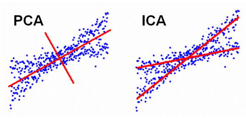
In other words ** A technique that axes in the direction of maximum independence when it can be assumed that the data are statistically independent and do not follow a normal distribution. The output will be independent data that does not follow a normal distribution (no linear or non-linear relationships) **
Difference between PCA and ICA (image)
 (Reference http://meg.aalip.jp/ICA/)
PCA implementation
PCA.py
import numpy as np
import matplotlib.pyplot as plt

from sklearn.decomposition import PCA
X = input_data #400 (number of data) x 300 (time series) data

#PCA execution
pca = PCA(n_components=20, random_state=0)#Make 20 bases (components)
feature = pca.fit_transform(X)
PCA_comp =  pca.components_ #Basis matrix

#Restore 0th data with 20 components
plt.figure(figsize = (12, 2))
plt.plot(X[0], label="data")#0th data
plt.plot(np.dot(feature[0], PCA_comp).T, label="reconstruct")#Restored 0th data
plt.legend()

Implementation of ICA
ICA.py
import numpy as np
import matplotlib.pyplot as plt

from sklearn.decomposition import FastICA
X = input_data #400 (number of data) x 300 (time series) data

#Implementation of ICA
ICA = FastICA(n_components=20, random_state=0)#Make 20 bases (components)
X_transformed = ICA.fit_transform(X)
A_ =  ICA.mixing_.T #Mixed matrix

#Restore 0th data with 20 components
plt.figure(figsize = (12, 2))
plt.plot(X[0], label="data")#0th data
plt.plot(np.dot(X_transformed[0], A_), label="reconstruct")#Restored 0th data
plt.legend()

in conclusion
This time, I have summarized PCA and ICA as a memorandum. I thought it would be okay because I was able to implement it for the time being, but I think I need to acquire more theoretical knowledge for the future. I would like to add about NMF (Non-negative matrix factorization).
reference
・ Dimension reduction method (summary and implementation) PCA, LSI (SVD), LDA, ICA
Recommended Posts