How to use OpenGoddard 1-python library for nonlinear optimal control and orbit generation

How to use Open Goddard 1

OpenGoddard is a python library for finding numerical solutions to my nonlinear optimal control problems.

https://github.com/istellartech/OpenGoddard https://istellartech.github.io/OpenGoddard/

Here, an example of actual usage is explained.

How to use OpenGoddard 1 ← Now here How to use OpenGoddard 2 How to use OpenGoddard 3 How to use OpenGoddard 4

Optimization problem

Optimal control problems are constrained optimization problems, and optimization problems are [wikipedia](https://ja.wikipedia.org/wiki/%E6%9C%80%E9%81%A9%E5% As described in 8C% 96% E5% 95% 8F% E9% A1% 8C), there are multiple types depending on the shape of the evaluation function and the presence or absence of constraints. OpenGoddard is a library for solving nonlinear programming (NLP) = nonlinear optimal control problems. Nonlinear Optimal Control Problem = Nonlinear Programming → [Sequential Quadratic Programming](https://ja.wikipedia.org/wiki/%E9%80%90%E6%AC%A1%E4%BA%8C%E6% I am doing the solution with AC% A1% E8% A8% 88% E7% 94% BB% E6% B3% 95) (sequential quadratic programming, SPQ). In OpenGoddard, when the evaluation function, equation of motion, constraint condition and calculation condition are entered, the constraint condition of the method called pseudospectral method is added and it is in Scipy of python. It is solved by the sequential quadratic programming solver (SLSQP). The user only needs to enter the evaluation function, equation of motion (ordinary differential equation), constraint condition, and calculation condition without looking at the method inside.

Brachistochrone problem

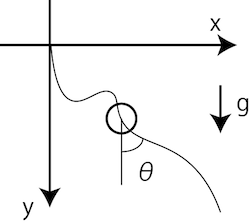
A classic example of an optimal control problem, taking the famous brachistochrone problem as an example. Find the curve (orbit) that allows the ball (mass point) to reach the farthest distance in the presence of gravity, assuming that there is no friction or air resistance. If you google it, it will come out, but this curve will be a cycloid curve. Simple examples such as the typical brachistochrone problem usually use the indirect method (variational method). This is because it is easy to obtain an analytical solution by converting mathematical expressions. However, with abundant computer resources, the direct method is more realistic for "practical use". So, I will use my open Goddard, which is a library of the direct method, especially the pseudo-spectral method.

As written in the README of github, write the python script in the following flow.

1. Description of method and variable of object class that optimizes orbit
2. Function of equation of motion
3. Constraint function
4. Function of evaluation function
5. Problem instance generation
6. Generating an object instance that optimizes the trajectory
7. Unit setting for normalization of optimization variables (optional)
8. Initial value estimation and installation (optional)
9. Function specification and knotting condition specification
10. solve
11. Post process (visualization)

In particular, the part where the equation of motion, constraints, and evaluation function are written down must be considered in advance.

Equation of motion

The equation of motion is as follows. (Note that the formula differs depending on the literature depending on how to take the angle)

\dot{x} = v \sin{\theta} \\
\dot{y} = v \cos{\theta} \\
\dot{v} = g \cos{\theta} 

Restraint condition

Constraint conditions give hints such as initial conditions, termination conditions, and things that are not physically strange. Here, the condition is that $ x = 1 $ is reached and y can be anywhere.

\theta \geq 0 \\
[x(t_0), y(t_0), v(t_0), t0, x(t_f)] = [0, 0, 0, 0, 1] \\
t_f \geq 0

Evaluation function

Put in the function to minimize. Here, we want to find the route in the "shortest time", so we want to minimize the time.

J = t_f

result

To solve the optimization problem, it is necessary to initialize the state variables and control variables. If no initial value is set, all will be initialized as 0. If you enter a value that is too strange, the solution will diverge. In particular, if you enter the initial value that violates the zero percent or the restraint condition, the solution cannot be obtained.

Brachistochrone problem with orbital restraint

To understand the power of the direct method, let's add some additional conditions to the brachistochrone problem. Let's add the condition that there is an area (wall) where the ball (mass point) should not enter. Put the following in the constraint condition.

y \leq x \tan{\theta_0} + h_0

On the other hand, it can be solved by the variational method, but the analytical solution will not come out unless the mathematical formula is tampered with. Like OpenGoddard, the direct method is a numerical solution that is definitely not optimal like the analytical solution, but the solution is easy to come up with. However, please note that it is not a global optimum solution, but a local optimum solution. (It is not implemented as of v1.0.0, but there is also a method that can confirm the optimum)

result

You can see that the orbit is made while observing the restraint condition of the wall. This is different from the analytical solution solved by the variational method. This is due to the convergence threshold or insufficient number of division points.

The problem of connecting Tokyo and Osaka with a tunnel without friction and air resistance

As an actual application (?) Of the brachistochrone problem, imagine the section between Tokyo and Osaka, calculate what kind of tunnel should be dug to arrive at the fastest speed with a gravitational acceleration of 9.8 m / s2 and no friction and air resistance at a distance of 600 km. I will try.

I will change the distance to 600km and calculate as it is.

class Ball:
    def __init__(self):
        self.g = 9.8  # gravity [m/s2]
        self.l = 600000  # goal [m]
        self.h = 300000  # depth limit [m]

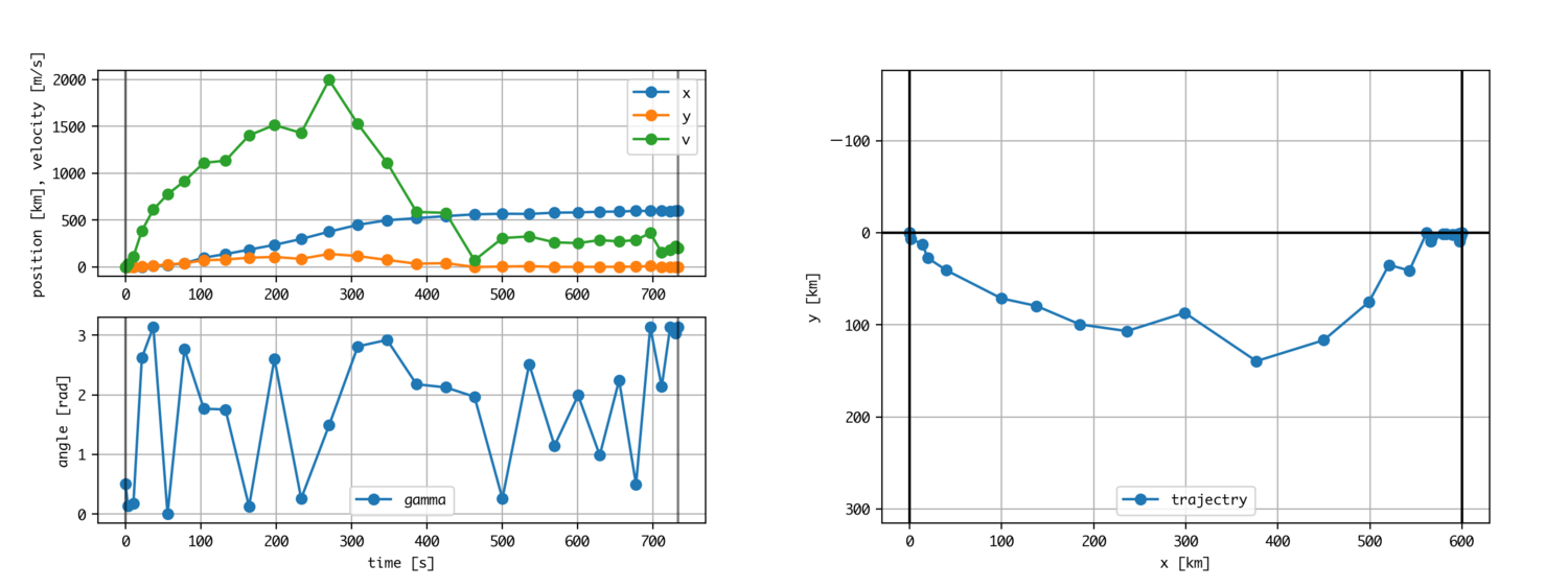
It was no good. The value of the control variable is fluttering and the result is not decent. Why? This is due to the variables being calculated internally.

prob.plot()

If you execute the above command on ipython or jupyter notebook after execution, the plot method of the Problem instance of OpenGoddard.optimize will be called, and you can visualize the values of the variables inside the optimization solver.

From left to right, it means state variables, control variables, and time (points). The leftmost part is the value of x. The order of values is hundreds of thousands. On the other hand, v is several thousand, and the value of the path angle θ is around 0 to 3. Sequential quadratic solvers are in a bad mood if the order of each variable is not correct. The reason is that the computer is trying to minimize the evaluation function by playing with the internal variables that are visualized without knowing the meaning of the variables, but if there are variables that are too effective and too ineffective for the evaluation function, it will not work.

Therefore, normalize the variables to order them. Set the state variables, control variables, and time so that the orders are aligned. A good rule of thumb is to keep the variables between -10 and 10.

unit_x = 300000
unit_y = 100000
unit_t = 100
unit_v = unit_x / unit_t
prob.set_unit_states_all_section(0, unit_x)
prob.set_unit_states_all_section(1, unit_y)
prob.set_unit_states_all_section(2, unit_v)
prob.set_unit_controls_all_section(0, 1.0)
prob.set_unit_time(unit_t)

The internal variables are now normalized.

This will give you a solution. It arrived in 10 minutes and 20 seconds with a maximum depth of 183 km and a maximum speed of Mach 5.5 (1893 m / s). In this tunnel, it is necessary to withstand almost free fall up to about 100 km underground, and since the deepest hole dug by human beings seems to be 12 km, it is necessary to dig more than 10 times that. Well, sorry, unrealistic.