2 . There are two types of sample search data for ChemTHEATER, measured data and samples, but this time we will use both.
The ChemTHEATER operation manual can be obtained from the ChemTHEATER Wiki site .
The simple operation guide is as follows.
- Click "Sample Search" on the menu bar from the top page of ChemTEHATRE.
- Select "Biotic --Mammals --Marine mammals" from the "Sample Type" pull-down menu.
- Select the scientific name of finless porpoise "Neophocaena phocaenoides" from the pull-down menu of "Scientific Name".
- Click the "Search" button.
- Click the "Export samples (TSV)" button to export the sample list, and the "Export measured data (TSV)" button to export the measured value list as tab-delimited text files.
- Save the exported file in any directory and use it for subsequent analysis.
data_file = "measureddata_20190826061813.tsv"    #Change the string entered in the variable to the tsv file name of your measured data
chem = pd.read_csv(data_file, delimiter="\t")
chem = chem.drop(["ProjectID", "ScientificName", "RegisterDate", "UpdateDate"], axis=1)    #Remove duplicate columns when joining with samples later
sample_file = "samples_20190826061810.tsv"    #Change the string entered in the variable to the tsv file name of your samples
sample = pd.read_csv(sample_file, delimiter="\t")
The downloaded TSV file is read by the pandas function (read_csv). At this time, it is necessary to change the path of each file ("data_file" and "sample_file" in the upper cell) to a file name suitable for each environment. In the sample code, the data file is written in the same directory as the notebook.
## Chap.3 Data preparation
The data handled this time is a compilation of measurement results of various chemical substances. Furthermore, the measurement results and the sample data are scattered. In other words, it is difficult to handle as it is, so it is necessary to shape it into a shape that is easy to handle. Specifically, the following operations are required.
Combine sample with - chem.
- Extract only the measurement data of the chemical substances handled this time.
- Delete columns that are not needed for visualization.
Sec.3-1 Extraction of necessary data
First, process 1 and 2 shown above.
Bonding is the work of adding a sample data frame (sample) of a sample of each chemical substance to the data frame (chem) of each chemical substance. Here, the sample data corresponding to the Sample ID of each chem data is attached to the right side of the chem.
df = pd.merge(chem, sample, on="SampleID")
In the data handled this time, each chemical substance is classified in a fairly detailed manner. You may visualize the measurement results for each chemical substance, but this time we want to visualize the outline of the measurement results so that you can see at a glance, so we will extract the data of the total value of each group when the chemical substances are roughly classified. ..
In addition, the data handled this time contains a mixture of two different units. Since it is meaningless to compare different units, this time we will divide the data for each unit. In the code below, Unit is specified in the first line of each, and the lipid and wet conversions are extracted, and then only the variables starting with Σ are extracted. In the second line, variables that start with Σ but are not the total value of chemical concentration are actually deleted from the data.
data_lipid = df[(df["Unit"] == "ng/g lipid") & df["ChemicalName"].str.startswith("Σ")]
data_lipid = data_lipid[(data_lipid["ChemicalName"] != "ΣOH-penta-PCB") & (data_lipid["ChemicalName"] != "ΣOH-hexa-PCB")
                        & (data_lipid["ChemicalName"] != "ΣOH-hepta-PCB") &  (data_lipid["ChemicalName"] != "ΣOH-octa-PCB")]
data_wet = df[(df["Unit"] == "ng/g wet") & df["ChemicalName"].str.startswith("Σ")]
data_wet = data_wet[(data_wet["ChemicalName"] != "ΣOH-penta-PCB") & (data_wet["ChemicalName"] != "ΣOH-hexa-PCB")
                    & (data_wet["ChemicalName"] != "ΣOH-hepta-PCB") &  (data_wet["ChemicalName"] != "ΣOH-octa-PCB")]
Data outline
This is the result of processing with Sec.3-1 (only for those whose unit is ng / g lipid). By deleting unnecessary data, only 131 data for 6 chemical substances could be extracted.
```python
data_lipid
```
|
MeasuredID |
SampleID |
ChemicalID |
ChemicalName |
ExperimentID |
MeasuredValue |
AlternativeData |
Unit |
Remarks_x |
ProjectID |
... |
| 4371 |
24782 |
SAA001903 |
CH0000033 |
ΣDDTs |
EXA000001 |
68000.0 |
NaN |
ng/g lipid |
NaN |
PRA000030 |
... |
| 4372 |
24768 |
SAA001903 |
CH0000096 |
ΣPCBs |
EXA000001 |
5700.0 |
NaN |
ng/g lipid |
NaN |
PRA000030 |
... |
| 4381 |
24754 |
SAA001903 |
CH0000138 |
ΣPBDEs |
EXA000001 |
170.0 |
NaN |
ng/g lipid |
NaN |
PRA000030 |
... |
| 4385 |
24902 |
SAA001903 |
CH0000142 |
ΣHBCDs |
EXA000001 |
5.6 |
NaN |
ng/g lipid |
NaN |
PRA000030 |
... |
| 4389 |
24810 |
SAA001903 |
CH0000146 |
ΣHCHs |
EXA000001 |
1100.0 |
NaN |
ng/g lipid |
NaN |
PRA000030 |
... |
| ... |
... |
... |
... |
... |
... |
... |
... |
... |
... |
... |
... |
| 4812 |
25125 |
SAA001940 |
CH0000152 |
ΣCHLs |
EXA000001 |
160.0 |
NaN |
ng/g lipid |
NaN |
PRA000030 |
... |
| 4816 |
25112 |
SAA001941 |
CH0000033 |
ΣDDTs |
EXA000001 |
9400.0 |
NaN |
ng/g lipid |
NaN |
PRA000030 |
... |
| 4817 |
25098 |
SAA001941 |
CH0000096 |
ΣPCBs |
EXA000001 |
1100.0 |
NaN |
ng/g lipid |
NaN |
PRA000030 |
... |
| 4818 |
25140 |
SAA001941 |
CH0000146 |
ΣHCHs |
EXA000001 |
41.0 |
NaN |
ng/g lipid |
NaN |
PRA000030 |
... |
| 4819 |
25126 |
SAA001941 |
CH0000152 |
ΣCHLs |
EXA000001 |
290.0 |
NaN |
ng/g lipid |
NaN |
PRA000030 |
... |
131 rows × 74 columns
Sec.3-2 Delete unnecessary columns
Next, delete unnecessary columns. In general, if the amount of information is the same, it is better to handle a small amount of data, so it is better to delete unnecessary data. In the data frame handled this time, there are many blanks without data. This is treated as N / A (floating point number) on python, and although there is no information, it consumes a certain amount of space. Therefore, all N / A columns (columns without information) are deleted from the data frame.
```python
data_lipid = data_lipid.dropna(how='all', axis=1)
data_wet = data_wet.dropna(how='all', axis=1)
```
Data outline
This is the result of processing Sec.3-2. It can be seen that the number of columns (the value of columns appearing at the bottom of the table) is considerably smaller than the result of Sec.3-1.
```python
data_lipid
```
|
MeasuredID |
SampleID |
ChemicalID |
ChemicalName |
ExperimentID |
MeasuredValue |
Unit |
ProjectID |
SampleType |
TaxonomyID |
... |
| 4371 |
24782 |
SAA001903 |
CH0000033 |
ΣDDTs |
EXA000001 |
68000.0 |
ng/g lipid |
PRA000030 |
ST004 |
34892 |
... |
| 4372 |
24768 |
SAA001903 |
CH0000096 |
ΣPCBs |
EXA000001 |
5700.0 |
ng/g lipid |
PRA000030 |
ST004 |
34892 |
... |
| 4381 |
24754 |
SAA001903 |
CH0000138 |
ΣPBDEs |
EXA000001 |
170.0 |
ng/g lipid |
PRA000030 |
ST004 |
34892 |
... |
| 4385 |
24902 |
SAA001903 |
CH0000142 |
ΣHBCDs |
EXA000001 |
5.6 |
ng/g lipid |
PRA000030 |
ST004 |
34892 |
... |
| 4389 |
24810 |
SAA001903 |
CH0000146 |
ΣHCHs |
EXA000001 |
1100.0 |
ng/g lipid |
PRA000030 |
ST004 |
34892 |
... |
| ... |
... |
... |
... |
... |
... |
... |
... |
... |
... |
... |
... |
| 4812 |
25125 |
SAA001940 |
CH0000152 |
ΣCHLs |
EXA000001 |
160.0 |
ng/g lipid |
PRA000030 |
ST004 |
34892 |
... |
| 4816 |
25112 |
SAA001941 |
CH0000033 |
ΣDDTs |
EXA000001 |
9400.0 |
ng/g lipid |
PRA000030 |
ST004 |
34892 |
... |
| 4817 |
25098 |
SAA001941 |
CH0000096 |
ΣPCBs |
EXA000001 |
1100.0 |
ng/g lipid |
PRA000030 |
ST004 |
34892 |
... |
| 4818 |
25140 |
SAA001941 |
CH0000146 |
ΣHCHs |
EXA000001 |
41.0 |
ng/g lipid |
PRA000030 |
ST004 |
34892 |
... |
| 4819 |
25126 |
SAA001941 |
CH0000152 |
ΣCHLs |
EXA000001 |
290.0 |
ng/g lipid |
PRA000030 |
ST004 |
34892 |
... |
131 rows × 37 columns
Visualization of Chap.4 ΣDDTs
By processing in
Chap.3, we have prepared data for each of the two types of chemical substances. Here, we first visualize the degree of data distribution for ng / g lipids of ΣDDTs. </ p>
Sec.4-1 Data preparation
First, for visualization, ΣDDTs data is extracted from data_lipid.
```python
data_ddt = data_lipid[data_lipid["ChemicalName"] == "ΣDDTs"]
ddt_vals = data_ddt.loc[:, "MeasuredValue"]
data_ddt
```
|
MeasuredID |
SampleID |
ChemicalID |
ChemicalName |
ExperimentID |
MeasuredValue |
Unit |
ProjectID |
SampleType |
TaxonomyID |
... |
| 4371 |
24782 |
SAA001903 |
CH0000033 |
ΣDDTs |
EXA000001 |
68000.0 |
ng/g lipid |
PRA000030 |
ST004 |
34892 |
... |
| 4401 |
24783 |
SAA001904 |
CH0000033 |
ΣDDTs |
EXA000001 |
140000.0 |
ng/g lipid |
PRA000030 |
ST004 |
34892 |
... |
| 4431 |
24784 |
SAA001905 |
CH0000033 |
ΣDDTs |
EXA000001 |
140000.0 |
ng/g lipid |
PRA000030 |
ST004 |
34892 |
... |
| 4461 |
24785 |
SAA001906 |
CH0000033 |
ΣDDTs |
EXA000001 |
130000.0 |
ng/g lipid |
PRA000030 |
ST004 |
34892 |
... |
| 4491 |
24786 |
SAA001907 |
CH0000033 |
ΣDDTs |
EXA000001 |
280000.0 |
ng/g lipid |
PRA000030 |
ST004 |
34892 |
... |
5 rows × 37 columns
Sec.4-2 Basic statistics
Since the data was extracted in Sec.4-1, the basic statistics are calculated in order to grasp the characteristics of this data set. Basic statistics are some statistics that summarize a dataset. This time, the total number of data, mean, standard deviation, 1st quartile, median, 3rd quartile, minimum value, and maximum value are calculated.
```python
count = ddt_vals.count()
mean = ddt_vals.mean()
std = ddt_vals.std()
q1 = ddt_vals.quantile(0.25)
med = ddt_vals.median()
q3 = ddt_vals.quantile(0.75)
min = ddt_vals.min()
max = ddt_vals.max()
count, mean, std, q1, med, q3, min, max
```
(24, 102137.5, 81917.43357743236, 41750.0, 70500.0, 140000.0, 9400.0, 280000.0)
In the upper cell, the basic statistics are calculated individually, but pandas has a function that outputs the basic statistics together.
avgs = ddt_vals.describe()
avgs
count        24.000000
mean     102137.500000
std       81917.433577
min        9400.000000
25%       41750.000000
50%       70500.000000
75%      140000.000000
max      280000.000000
Name: MeasuredValue, dtype: float64
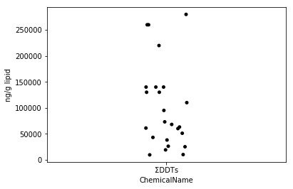
Sec.4-3 jitter plot
There is a scatter plot that plots all the data as a way to visualize how the data is scattered (Eguchi: Is this a jitter plot, not a scatter plot?). In Python, you can easily draw a jitter plot by using seaborn's stripplot function. Jitter plot is one of the good visualization methods that can easily describe each heaven by adding fluctuations to the dots even when the dots overlap.
fig = plt.figure()
ax = fig.add_subplot(1,1,1)
sns.stripplot(x="ChemicalName", y="MeasuredValue", data=data_ddt, color='black', ax=ax)  #Drawing of jitter plot
ax.set_ylabel("ng/g lipid")
plt.show()
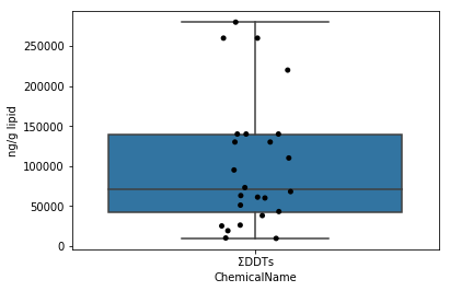
Sec.4-4 Box plot
Unlike Sec.4-3, the boxplot plots a summary of the dataset with basic statistics. Box plots can be drawn with seaborn's boxplot function. Here, by overwriting the boxplot on the jitter plot mentioned earlier, a diagram that makes it easier to understand the distribution of data is output.
fig = plt.figure()
ax = fig.add_subplot(1,1,1)
sns.stripplot(x="ChemicalName", y="MeasuredValue", data=data_lipid[data_lipid["ChemicalName"] == "ΣDDTs"], color='black', ax=ax) #Drawing of jitter plot
sns.boxplot(x="ChemicalName", y="MeasuredValue", data=data_lipid[data_lipid["ChemicalName"] == "ΣDDTs"], ax=ax) #Drawing a box plot
ax.set_ylabel("ng/g lipid")
plt.show()
Visualization of each chemical data of finless porpoise ( Neophocaena phocaenoides </ i>)
In Chap.4, only the values of ΣDDTs were visualized. Apply it to visualize data_lipid and data_wet data.
### Sec.5-1 Box plot (application of Sec.4-4)
First, draw a graph for the data of data_lipid in the same way as Sec.4-4. Since the stripplot / boxplot function has a function to automatically classify the data by the column name to be assigned to the parameter x, the collected data can be directly assigned to the parameter data.
```python
fig = plt.figure()
ax = fig.add_subplot(1,1,1)
sns.stripplot(x="ChemicalName", y="MeasuredValue", data=data_lipid, color='black', ax=ax) #Drawing of jitter plot
sns.boxplot(x="ChemicalName", y="MeasuredValue", data=data_lipid, ax=ax) #Drawing a box plot
ax.set_ylabel("ng/g lipid")
plt.show()
```
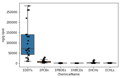
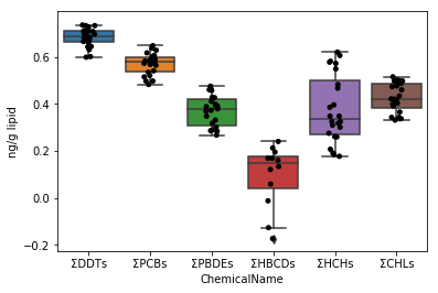
Sec.5-2 Improvement of Sec.5-1
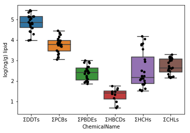
In the graph above, the ΣDDTs vary widely, so the y-axis spacing is wide. Therefore, the remaining 5 types of graphs are crushed and difficult to see. Therefore, the graph is made easier to see by taking the logarithm of the data values.
First, when taking the logarithm, the logarithm of 0 cannot be taken, so check if the data set contains 0. By using the in statement, the presence or absence of the corresponding value is returned as TRUE / FALSE.
0 in data_lipid.loc[:, "MeasuredValue"].values
False
Since we found that the dataset does not contain 0 in the upper cell, we can take the logarithmic value as it is.
```python
data_lipid.loc[:, "MeasuredValue"] = data_lipid.loc[:, "MeasuredValue"].apply(np.log10)
```
C:\Users\masah\Anaconda3\lib\site-packages\pandas\core\indexing.py:543: SettingWithCopyWarning:
A value is trying to be set on a copy of a slice from a DataFrame.
Try using .loc[row_indexer,col_indexer] = value instead

See the caveats in the documentation: http://pandas.pydata.org/pandas-docs/stable/indexing.html#indexing-view-versus-copy
  self.obj[item] = s
fig = plt.figure()
ax = fig.add_subplot(1,1,1)
sns.stripplot(x="ChemicalName", y="MeasuredValue", data=data_lipid, color='black', ax=ax) #Drawing of jitter plot
sns.boxplot(x="ChemicalName", y="MeasuredValue", data=data_lipid, ax=ax) #Drawing a box plot
ax.set_ylabel("log(ng/g) lipid")
plt.show()
Visualize
data_wet in the same way. First, if the dataset contains 0s, substitute 1/2 of the minimum value instead. Then take the logarithm and visualize it. </ p>
if 0 in data_wet.loc[:, "MeasuredValue"].values:
    data_wet["MeasuredValue"].replace(0, data_wet[data_wet["MeasuredValue"] != 0].loc[:, "MeasuredValue"].values.min() / 2) #Minimum value 1/Substitute 2
else:
    pass
data_lipid.loc[:, "MeasuredValue"] = data_lipid["MeasuredValue"].apply(np.log10)
data_lipid.loc[:, "Unit"] = "log(ng/g lipid)"
fig = plt.figure()
ax = fig.add_subplot(1,1,1)
sns.stripplot(x="ChemicalName", y="MeasuredValue", data=data_lipid, color='black', ax=ax)
sns.boxplot(x="ChemicalName", y="MeasuredValue", data=data_lipid, ax=ax)
ax.set_ylabel("log(ng/g lipid)")
plt.show()
footnote
1 It is a function of Juyter Notebook called "magic command", and it should be noted that it cannot be used in general python code.
2 Abbreviation for tab-separated values. It is a file format in which data is separated by TAB characters (at the left end of the keyboard). Suitable for holding table-shaped data. A similar file format is CSV (abbreviation for comma-separated values, separated by ", (comma)").
